Lecture 3. Markov semigroups and Dirichlet forms

Let (X, ℬ) be a measurable space. We say that (X, ℬ) is a good measurable space if there is a countable family generating ℬ and if every finite measure γ on (X × X, ℬ ⊗ ℬ) can be decomposed as

γ(dx dy) = k(x,dy) γ1(dx)

where γ1 is the projection of γ on the first coordinate and k is a kernel, i.e. k(x,·) is a finite measure on (X, ℬ) and x → k(x,A) is measurable for every A ∈ ℬ.

For instance, if X is a Polish space (or a Radon space) equipped with its Borel σ-field, then it is a good measurable space.

Throughout the lecture, we will consider (X, ℬ, μ) to be a good measurable space equipped with a σ-finite measure μ.

Contents

Markovian semigroups

Definition Let (Pt)t≥0 be a strongly continuous self-adjoint contraction semigroup on L2(X,μ). The semigroup (Pt)t≥0 is called Markovian if and only if for every f ∈ L2(X,μ) and t ≥ 0:

  1. f ≥ 0, a.e. ⇒ Ptf ≥ 0, a.e.

  2. f ≤ 1, a.e. ⇒ Ptf ≤ 1, a.e.

We note that if (Pt)t≥0 is Markovian, then for every f ∈ L2(X,μ) ∩ L∞(X,μ),

||Ptf||L∞(X,μ) ≤ ||f||L∞(X,μ).

As a consequence (Pt)t≥0 can be extended to a contraction semigroup defined on all of L∞(X,μ).

Definition A transition function {pt,t ≥ 0} on X is a family of kernelsnpt : X × ℬ → [0,1]

such that:

  1. For t ≥ 0 and x ∈ X, pt(x, ·) is a finite measure on X;
  2. For t ≥ 0 and A ∈ ℬ the application x → pt(x,A) is measurable;
  3. For s,t ≥ 0, a.e. x ∈ X and A ∈ ℬ,

    pt+s(x,A) = ∫X pt(y,A) ps(x,dy).

The relation above is often called the Chapman-Kolmogorov relation.

Theorem (Heat kernel measure)nLet (Pt)t≥0 be a strongly continuous self-adjoint contraction Markovian semigroup on L2(X,μ).nThere exists a transition function {pt,t ≥ 0} on X such that for every f ∈ L∞(X,μ) and a.e. x ∈ X

Ptf(x) = ∫X f(y) pt(x,dy) , t > 0.

This transition function is called the heat kernel measure associated to (Pt)t≥0.

The proof relies on the following lemma sometimes called the bi-measure theorem. A set function ν : ℬ ⊗ ℬ → [0,+∞) is called a bi-measure, if for every A ∈ ℬ, ν(A, ·) and ν(·, A) are measures.

Lemma If ν : ℬ ⊗ ℬ → [0,+∞) is a bi-measure, then there exists a measure γ on ℬ ⊗ ℬ such that for every A,B ∈ ℬ,

γ(A × B) = ν(A,B).

Proof of Theorem 7.3

We assume that μ is finite and let as an exercise the extension to σ-finite measures. For t > 0, we consider the set function

νt(A,B) = ∫X 1A Pt 1B dμ.

Since Pt is supposed to be Markovian, it is a bi-measure. From the bi-measure theorem, there exists a measure γt on ℬ ⊗ ℬ such that for every A,B ∈ ℬ,

γt(A × B) = νt(A,B) = ∫X 1A Pt 1B dμ.

The projection of γt on the first coordinate is (Pt1) dμ, thus from the measure decomposition theorem, γt can be decomposed as

γt(dx dy) = pt(x,dy) μ(dx)

for some kernel pt. One has then for every A,B ∈ ℬ

∫X 1A Pt 1B dμ = ∫A ∫B pt(x,dy) μ(dx),

from which it follows that for every f ∈ L∞(X,μ), and a.e. x ∈ X

Ptf(x) = ∫X f(y) pt(x,dy).

The relation

pt+s(x,A) = ∫X pt(y,A) ps(x,dy)

follows from the semigroup property.

Exercise Prove Theorem 7.3 if μ is σ-finite.

Exercise Show that for every non-negative measurable function F : X × X → ℝ,

∫X ∫X F(x,y) pt(x,dy) dμ(x) = ∫X ∫X F(x,y) pt(y,dx) dμ(y).

Definition Let (Pt)t≥0 be a strongly continuous self-adjoint contraction Markovian semigroup on L2(X,μ). We say that the semigroup {Pt}t∈[0,∞) admits a heat kernel if the heat kernel measures have a density with respect to μ, i.e. there exists a measurable function p : ℝ>0 × X × X → ℝ≥0, such that for every t > 0, a.e. x,y ∈ X, f ∈ L∞(X,μ),

Ptf(x) = ∫X pt(x,y) f(y) dμ(y).

If the heat kernel exists, we will often denote p(t,x,y) as pt(x,y) for t > 0 and a.e. x,y ∈ X.

Dirichlet forms

Definition A function v on X is called a normal contraction of the function u if for almost every x, y ∈ X,

|v(x)-v(y)| ≤ |u(x) – u(y)| and |v(x)| ≤ |u(x)|.

Definition Let (ℰ,ℱ = dom(ℰ)) be a densely defined closed quadratic form on L2(X,μ). The form ℰ is called a Dirichlet form if it is Markovian, that is, has the property that if u ∈ ℱ and v is a normal contraction of u then v ∈ ℱ and

ℰ(v,v) ≤ ℰ(u,u).

Exercise Show that a densely defined closed quadratic form on L2(X,μ) is Markovian if and only if for every u ∈ ℱ, (0 ∨ u) ∧ 1 ∈ ℱ and ℰ( (0 ∨ u) ∧ 1, (0 ∨ u) ∧ 1 ) ≤ ℰ(u,u).

Theorem Let (Pt)t≥0 be a strongly continuous self-adjoint contraction semigroup on L2(X,μ). Then, (Pt)t≥0 is a Markovian semigroup if and only if the associated closed symmetric form on L2(X,μ) is a Dirichlet form.

Proof

Let (Pt)t≥0 be a strongly continuous self-adjoint contraction Markovian semigroup on L2(X,μ). There exists a transition function {pt, t ≥ 0} on X such that for every u ∈ L∞(X,μ) and a.e. x ∈ X

Ptu(x) = ∫X u(y) pt(x,dy), t > 0.

Denote

kt(x) = Pt1(x) = ∫X pt(x,dy).

We observe that from the Markovian property of Pt, we have 0 ≤ kt ≤ 1 a.e.
We have then

1/2 ∫X ∫X (u(x) – u(y))2 pt(x,dy) dμ(x) = ∫X u(x)2 kt(x)dμ(x) – ∫X u(x) Ptu(x) dμ(x).

Therefore,

⟨u – Ptu, u⟩ = 1/2 ∫X ∫X (u(x) – u(y))2 pt(x,dy) dμ(x) + ∫X u(x)2 (1 – kt(x)) dμ(x).

Let us now assume that u ∈ ℱ and that v is a normal contraction of u. One has

∫X ∫X (v(x) – v(y))2 pt(x,dy) dμ(x) ≤ ∫X ∫X (u(x) – u(y))2 pt(x,dy) dμ(x)

and

∫X v(x)2 (1 – kt(x)) dμ(x) ≤ ∫X u(x)2 (1 – kt(x)) dμ(x).

Therefore,

⟨v – Ptv,v⟩ ≤ ⟨u – Ptu,u⟩

Since u ∈ ℱ, one knows that (1/t)⟨u – Ptu,u⟩ converges to ℰ(u) when t → 0. Since (1/t)⟨v – Ptv,v⟩ is non-increasing and bounded it does converge when t → 0. Thus v ∈ ℱ and

ℰ(v) ≤ ℰ(u).

One concludes that ℰ is Markovian.

Now, consider a Dirichlet form ℰ and denote by Pt the associated semigroup in L2(X,μ) and by A its generator.
The main idea is to first prove that for λ > 0, the resolvent operator (λId – A)-1 preserves the positivity of function. Then, we may conclude by the fact that for f ∈ L2(X,μ), in the L2(X,μ) sense

Ptf = limn → +∞ (Id – t/n A)-nf.

Let λ > 0. We consider on ℱ the norm

||f||2λ = ||f||2L2(X,μ) + λℰ(f,f).

From the Markovian property of ℰ, if u ∈ ℱ, then |u| ∈ ℱ and

ℰ(|u|, |u|) ≤ ℰ(u, u).

We consider the bounded operator

Rλ = (Id – λA)-1

that goes from L2(X,μ) to 𝒟(A) ⊂ ℱ. For f ∈ ℱ and g ∈ L2(X,μ) with g ≥ 0, we have

⟨|f| , Rλ g⟩λ = ⟨|f| , Rλg⟩L2(X,μ) – λ⟨|f| , ARλ g⟩L2(X,μ)

= ⟨|f|, (Id – λA) Rλ g⟩L2(X,μ)

=⟨|f|, g⟩L2(X,μ)

≥ |⟨f, g⟩L2(X,μ)|

≥ |⟨f , Rλg⟩λ|.

Moreover, from inequality above, for f ∈ ℱ,

|||f|||λ2 = |||f| ||2L2(X,μ) + λℰ(|f|,|f|)

≤ ||f||2L2(X,μ) + λℰ(f,f)

≤ ||f||λ2.

By taking f = Rλ g in the two above sets of inequalities, we draw the conclusion

|⟨Rλg, Rλg⟩λ| ≤ ⟨|Rλg| , Rλg⟩λ ≤ |||Rλg|||λ ||Rλg||λ ≤ |⟨Rλg, Rλg⟩λ|.

The above inequalities are therefore equalities which implies

Rλg = |Rλg|.

As a conclusion if g ∈ L2(X,μ) is a.e. ≥ 0, then for every λ > 0, (Id – λA)-1g ≥ 0 a.e.. Thanks to the spectral theorem, in L2(X,μ),

Ptg = limn → +∞ (Id – t/n A)-ng.

By passing to a subsequence that converges pointwise almost surely, we deduce that Ptg ≥ 0 almost surely.

The proof of

f ≤ 1, a.e. ⇒ Ptf ≤ 1, a.e.

follows the same lines:

  1. The first step is to observe that if 0 ≤ f ∈ ℱ, then 1 ∧ f ∈ ℱ and moreover

ℰ(1 ∧ f, 1 ∧ f) ≤ ℰ(f,f).

2. Let f ∈ L2(X,μ) satisfy 0 ≤ f ≤ 1 and set g = Rλf = (Id – λA)-1f ∈ ℱ and h = 1 ∧ g. According to the first step, h ∈ ℱ and ℰ(h,h) ≤ ℰ(g,g). Now, we observe that:

||g – h||λ2 = ||g||λ2 – 2⟨g,h⟩λ + ||h||λ2

= ⟨Rλf,f⟩L2(X,μ) – 2⟨f,h⟩L2(X,μ) + ||h||2L2(X,μ) + λℰ(h,h)

= ⟨Rλf,f⟩L2(X,μ) – ||f||2L2(X,μ) + ||f – h||2L2(X,μ) + λℰ(h,h)

≤ ⟨Rλf,f⟩L2(X,μ) – ||f||2L2(X,μ) + ||f – g||2L2(X,μ) + λℰ(g,g) = 0.

As a consequence g = h, that is 0 ≤ g ≤ 1.

3. The previous step shows that if f ∈ L2(X,μ) satisfies 0 ≤ f ≤ 1 then for every λ > 0, 0 ≤ (Id – λL)-1 f ≤ 1. Thanks to the spectral theorem, in L2(X,μ),

Ptf = limn → +∞ (Id – t/n L)-nf.

By passing to a subsequence that converges pointwise almost surely, we deduce that 0 ≤ Ptf ≤ 1 almost surely.

Posted in Dirichlet forms at NYU | Tagged , | Leave a comment

Lecture 2. Quadratic forms in Hilbert spaces

Contents

Quadratic forms and generators

Definition A quadratic form ℰ on H is a non-negative definite, symmetric bilinear form 𝒟(ℰ) × 𝒟(ℰ) → ℝ, where 𝒟(ℰ) is a dense subspace of H. A quadratic form ℰ on H is said to be closed if 𝒟(ℰ) equipped with the norm

‖f‖𝒟(ℰ)2= ‖f‖2 + ℰ(f,f)

is a Hilbert space. A quadratic form ℰ on H is said to be closable it admits a closed extension, i.e. there exists a closed quadratic form ℰ’ such that 𝒟(ℰ) ⊂ 𝒟(ℰ’) and ℰ’ coincides with ℰ on 𝒟(ℰ) × 𝒟(ℰ).

Lemma A quadratic form ℰ is closable if and only if for any sequence fn in 𝒟(ℰ) such that fn → 0 in H and ℰ(fn – fm, fn – fm) → 0 when n, m → +∞ one has ℰ(fn, fn) → 0.

Proof

On 𝒟(ℰ), let us consider the following norm

||f||ℰ2 = ||f||2 + ℰ(f, f).

By completing 𝒟(ℰ) with respect to this norm, we get an abstract Hilbert space (Hℰ,⟨⋅,⋅⟩ℰ). Since for f ∈ 𝒟(ℰ), ||f|| ≤ ||f||ℰ, the injection map ι : (𝒟(ℰ), || · ||ℰ) → (H, || · ||) is continuous and it may therefore be extended into a continuous map ῑ : (Hℰ, || · ||ℰ) → (H, || · ||). Let us show that ̄ι is injective so that Hℰ may be identified with a subspace of H. So, let f ∈ Hℰ such that ῑ(f) = 0. We can find a sequence fn ∈ 𝒟(ℰ), such that || fn – f ||ℰ → 0 and || fn || → 0. We have then

||f||ℰ2 = limn → + ∞ ⟨fn, fn⟩ℰ

= limn → + ∞ ⟨fn,fn⟩ + ℰ(fn, fn)

= 0,

thus f=0 and ῑ is injective. Therefore, Hℰ may be identified with a subspace of H and the quadratic form on H defined by

ℰ'(f) = ||f||ℰ2 – ||f||2, f ∈ Hℰ

is closed because (Hℰ,⟨⋅,⋅⟩ℰ) is a Hilbert space and obviously is an extension of ℰ.

If a quadratic form ℰ is closable, then its minimal closed extension is called the closure of ℰ. In that case, one can easily check that the closure of ℰ is actually the quadratic form ℰ constructed in the previous proof.

Theorem Let ℰ be a closed symmetric non-negative bilinear form on H. There exists a unique densely defined non-positive self-adjoint operator A on H defined by

𝒟(A) = {f ∈ H, ∃g ∈ H, ∀h ∈ H, ℰ(f,h) = -⟨h,g⟩}

Af = g.

The operator A is called the generator of ℰ. Conversely, if A is a densely defined non-positive self-adjoint operator on H, one can define a closed symmetric non-negative bilinear form ℰ on H by

𝒟(ℰ) = 𝒟((-A)1/2), ℰ(f,g) = ⟨(-A)1/2f,(-A)1/2g⟩.

Proof

Let ℰ be a closed symmetric non-negative bilinear form on H. As usual, we denote by ℱ the domain of ℰ. We note that for λ > 0, ℱ equipped with the norm (||f||2 + λℰ(f))1/2 is a Hilbert space because ℰ is closed. From the Riesz representation theorem, there exists then a linear operator Rλ :H → ℱ such that for every f ∈ H, g ∈ ℱ

⟨f,g⟩ = λ⟨Rλ f , g⟩ + ℰ(Rλ f,g).

From the definition, the following properties are then easily checked:

  1. ||Rλf|| ≤ (1/λ) ||f|| (apply the definition of Rλ with g = Rλf and then use the Cauchy-Schwarz inequality);
  2. For every f,g ∈ H, ⟨Rλf , g⟩ = ⟨f , Rλg⟩;
  3. Rλ1 – Rλ2 + (λ1 – λ2)Rλ1Rλ2 = 0;
  4. For every f ∈ H, limλ → +∞ || λRλf -f || = 0.

We then claim that Rλ is invertible. Indeed, if Rλf = 0, then for α > λ , one has from 3, Rαf = 0. Therefore f = limα → +∞ Rαf = 0. Denote then

Af = λf – Rλ-1f,

and 𝒟(A) is the range of Rλ. It is straightforward to check that A does not depend on λ. The operator A is a densely defined self-adjoint operator that satisfies the properties stated in the theorem (Exercise !).

Conversely, if A is a densely defined non-positive self-adjoint operator on H, then (-A)1/2 is a densely defined self-adjoint operator and the quadratic form

ℰ(f,g) := ⟨(-A)1/2f, (-A)1/2g⟩

is closed and densely defined on 𝒟((-A)1/2).

Exercise Prove the properties 1,2,3,4 of the previous proof.

In practice, the following lemma is often useful to construct closed quadratic forms and easily follows from the previous results.

Lemma Let A be a densely defined non-positive symmetric operator 𝒟(A) → H. The quadratic form

ℰ(f,g) = -⟨f, Ag⟩, f,g ∈ 𝒟(A)

is closable and the generator of its closure is a self-adjoint extension of A.

Semigroups and quadratic forms

Theorem Let (Pt)t≥0 be a strongly continuous self-adjoint contraction semigroup on H. One can define a closed quadratic form on H by

ℰ(f,f) := limt → 0 ⟨(Id – Pt)/t f, f⟩,

where the domain of this form is the set of f‘s for which the limit exists. The quadratic form ℰ is called the quadratic form associated to the semigroup (Pt)t≥0.

Proof

Let A be the generator of the semigroup (Pt)t ≥ 0. We use spectral theorem to represent A as

U-1 A U g(x) = -λ(x) g(x),

so that

U-1 Pt U g(x) = e-tλ(x) g(x).

We then note that for every g ∈ L2(Ω,ν),

⟨(Id – Pt)/t Ug, Ug⟩ = ∫Ω (1 – e-tλ(x))/t g(x)2 dν(x).

This proves that for every f ∈ H, the map t → ⟨(Id – Pt)/t f, f⟩ is non-increasing. Therefore, the limit limt → 0 ⟨(Id – Pt)/t f, f⟩ exists if and only if ∫Ω (U-1f)2(x) λ(x) dν(x) < +∞, which is equivalent to the fact that f ∈ 𝒟((-A)1/2). In which case we have

limt → 0 ⟨(Id – Pt)/t f, f⟩ = ||(-A)1/2f||2.

Since (-A)1/2 is a densely defined self-adjoint operator, the quadratic form

ℰ(f) := ||(-A)1/2f||2

is closed and densely defined on ℱ := 𝒟((-A)1/2).

A first example: The Dirichlet energy on an open set Ω ⊂ ℝn

Let Ω ⊂ ℝn be an open connected set. We do not assume any regularity on the boundary of Ω. Classically, one can define the (1,2) Sobolev space

W1,2(Ω) = {f ∈ L2(Ω) : ∂f/∂xi ∈ L2(Ω)}

where the derivatives ∂u/∂xi are understood in the weak sense. The quadratic form

ℰ(f,g) = ∫Ω ⟨∇f, ∇g⟩ dx = ∑i=1n ∫Ω ∂f/∂xi ∂g/∂xi dx

with domain W1,2(Ω) is then a closed densely defined quadratic form on L2(Ω) since it is well-known that the Sobolev norm

||f||2W1,2(Ω) = ||f||2L2(Ω) + ||∇f||2L2(Ω)

is complete. The generator of the form ℰ is called the Neumann Laplacian on Ω.

On the other hand, let

Δ = ∑i=1n ∂2/∂xi2

be the usual Laplacian on ℝn, the derivatives being understood in the ordinary sense, and Cc∞(Ω) be the set of smooth functions with a compact support included in Ω. Then, from a lemma, the quadratic form

ℰ0(f,g) = -∫Ω f Δg dx

with domain Cc∞(Ω) is closable. The domain of the closure of ℰ0 is the Sobolev space W01,2(Ω) and the generator of the closure of ℰ0 is called the Dirichlet Laplacian on Ω.

Notice that both the Neumann and the Dirichlet Laplacian are self-adjoint extensions of the Laplacian Δ with domain Cc∞(Ω). In general, the Neumann and Dirichlet Laplacian do not coincide. For instance if the boundary of Ω is smooth, then smooth functions in the domain of the Neumann Laplacian have vanishing normal derivatives while smooth functions in the domain of the Dirichlet Laplacian vanish on the boundary of u.

Posted in Dirichlet forms at NYU | Tagged , | Leave a comment

Lecture 1: Semigroups and generators

Contents

Preliminaries: Self-adjoint Operators

Let (H,⟨⋅,⋅⟩) be a Hilbert space with norm ‖f‖2=⟨f,f⟩ and let A be a H-valued densely defined operator on a domain 𝒟(A). We recall the following basic definitions.

  • The operator A is said to be closed if xn → x in H and Axn → y in H imply that y=Ax.
  • The operator A is said to be symmetric if for f,g ∈ 𝒟(A), ⟨f,Ag⟩ = ⟨Af,g⟩
  • The operator A is said to be non-negative symmetric operator if it is symmetric and if for f ∈ 𝒟(A), ⟨f,Af⟩ ≥ 0. It is said to be non-positive, if for f ∈ 𝒟(A), ⟨f,Af⟩ ≤ 0
  • The adjoint A* of A is an operator defined on the domain

    𝒟(A*) = {f ∈ H : ∃ c(f) ≥ 0, ∀ g ∈ 𝒟(A), |⟨f,Ag⟩| ≤ c(f)‖g‖}

    Since for f ∈ 𝒟(A*), the map g → ⟨f,Ag⟩ is bounded on 𝒟(A), it extends thanks to the Hahn-Banach theorem to H. The Riesz representation theorem allows then to define A* by the formula ⟨A*f,g⟩ = ⟨f,Ag⟩ where g ∈ 𝒟(A), f ∈ 𝒟(A*). Since 𝒟(A) is dense, A* is uniquely defined.

  • The operator A is said to be self-adjoint if it is symmetric and if 𝒟(A*) = 𝒟(A).

Let us observe that, in general, the adjoint A* is not necessarily densely defined, however it is readily checked that if A is a symmetric operator then, from Cauchy-Schwarz inequality, 𝒟(A) ⊂ 𝒟(A*). Thus, if A is symmetric, then A* is densely defined. The following result is often useful and classical.

Lemma  Let A : 𝒟(A) ⊂ H → H be an injective densely defined self-adjoint operator. Let us denote by 𝓡(A) the range of A. The inverse operator A-1 : 𝓡(A) → H is a densely defined self-adjoint operator.

A major result in functional analysis is the spectral theorem.

Theorem  (Spectral theorem) Let A be a non-negative self-adjoint operator on H. There is a measure space (Ω,ν), a unitary map U : L2(Ω,ν) → H and a non-negative real-valued measurable function λ on Ω such that

U-1 A U f (x) = λ(x) f(x)

for x ∈ Ω, Uf ∈ 𝒟(A). Moreover, given f ∈ L2(Ω,ν), Uf belongs to 𝒟(A) if only if ∫Ω λ2 f2 dν < +∞.

Definition  (Functional calculus) Let A be a non-negative self-adjoint operator on H. Let g : ℝ≥0 → ℝ be a Borel function. With the notations of the spectral theorem, one defines the operator g(A) by the requirement

U-1 g(A) U f (x) = g(λ(x)) f(x)

with 𝒟(g(A)) = {Uf, (g ∘ λ) f ∈ L2(Ω,ν) }.

Exercise  Show that if A is a non-negative self-adjoint operator on H and g is a bounded Borel function, then g(A) is a bounded operator on H.

Semigroups and generators

Definition  A strongly continuous self-adjoint contraction semigroup is a family of self-adjoint operators (Pt)t≥0 : H → H such that:

  1. For s, t ≥ 0, Pt ∘ Ps = Ps+t (semigroup property);
  2. For every f ∈ H, limt → 0 Pt f = f (strong continuity);
  3. For every f ∈ H and t ≥ 0, ‖Pt f‖ ≤ ‖f‖ (contraction property).

Theorem Let (Pt)t≥0 be a strongly continuous self-adjoint contraction semigroup on H. There exists a self-adjoint, non-positive, and densely defined operator A : 𝒟(A) → H where

𝒟(A) = {f ∈ H : limt → 0 (Ptf – f)/t exists}

such that for f ∈ 𝒟(A),

limt → 0 || (Ptf – f)/t – Af || = 0.

The operator A is called the generator of the semigroup (Pt)t≥0. We also say that A generates (Pt)t≥0. Conversely, if A is a densely defined non-positive self-adjoint operator on H, then it is the generator of the strongly continuous self-adjoint contraction semigroup on H defined as Pt = etA.

Proof

Let us consider the following bounded operators on H:

At = (1/t) ∫0t Ps ds

For f ∈ H and h > 0, we have

(1/t)(PtAhf – Ahf) = (1/ht) ∫0h (Ps+tf – Psf) ds

=(1/ht)[ ∫th+t Psf ds – ∫0h Psf ds ]

= (1/ht)[ ∫hh+t Psf ds + ∫th Psf ds – ∫0h Psf ds ]

= (1/ht) ∫0t (Ps+hf – Psf) ds

Therefore, we obtain

limt → 0 (1/t) (PtAhf – Ahf) = (1/h) (Phf – f)

This implies,

{Ahf : x ∈ H, h > 0} ⊂ {f ∈ H : limt → 0 (Ptf – f)/t exists}

Since limh → 0 Ah f = f, we deduce that

{f ∈ H : limt → 0 (Ptf – f)/t exists}

is dense in H. We can then consider

Af := limt → 0 (Ptf – f)/t,

which is of course defined on the domain

𝒟(A) = {f ∈ H : limt → 0 (Ptf – f)/t exists}.

The operator A is closed, indeed if fn → f and Afn → g then, using similar computations as before,

Ahg = 1/h ∫0h Psg ds = limn →+∞ 1/h ∫0h PsAfn ds

= limn →+∞ limt → 0 1/ht ∫0h Ps+t fn – Psfn ds

=limn →+∞ limt → 0 1/ht ∫0t Ps+h fn – Psfn ds

= limn →+∞ 1/h (Phfn – fn) = 1/h(Phf – f)

Taking then the limit as h → 0 yields y = Ax. We now prove that A is a non-positive self-adjoint operator. First, one has for every f ∈ H

⟨Af,f⟩ = limt → 0 ⟨(Ptf – f)/t , x⟩

= limt → 0 (⟨Ptf,f⟩ – ||f||2)/t

=limt → 0 (||Pt/2f||2 – ||f||2)/t ≤ 0

From its definition, it is plain that A is symmetric but proving self-adjointness is a little more involved. Let λ > 0. We will to prove that λId – A is a bijective operator D(A) → H whose inverse is self-adjoint and conclude with a previous lemma.

The formal Laplace transform formula

∫0+∞ e-λt etA dt = (λId – A)-1,

suggests that the operator

Rλ = ∫0+∞ e-λt Pt dt

is the inverse of λId – A. We show this is indeed the case. First, let us observe that Rλ is well-defined as a Riemann integral since t → Pt is continuous and ||Pt|| ≤ 1. We now show that for f ∈ H, Rλx ∈ 𝒟(A). For h > 0,

(Ph – Id)/h Rλ f = ∫0+∞ e-λt (Ph – Id)/h Pt f dt

= ∫0+∞ e-λt (Ph+t – Pt)/h f dt

= eλh∫h+∞ e-λs (Ps – Ps-h)/h f ds

= (eλh/h) (Rλf – ∫0h e-λs Psf ds – ∫h+∞ e-λs Ps-hf ds)

= ((eλh – 1)/h)Rλf – (eλh/h) ∫0h e-λs Psf ds

By letting h → 0, we deduce that Rλf ∈ 𝒟(A) and moreover

ARλf = λRλf – f.

Therefore we proved

(λId – A)Rλ = Id.

Furthermore, it is readily checked that, since A is closed, for f ∈ 𝒟(A),

A Rλf = A ∫0+∞ e-λt Ptf dt = ∫0+∞ e-λt APtf dt = ∫0+∞ e-λt PtAf dt = RλAf.

We therefore conclude

(λId – A)Rλ = Rλ(λId – A) = Id.

Thus,

Rλ = (λId – A)-1,

The operator ∫0+∞ e-λt Pt dt is seen to be self-adjoint (it is symmetric and bounded), thus (λId – A)-1 is also self-adjoint. From the previous lemma, we deduce that λId – A is self-adjoint, from which we conclude that A is self-adjoint (exercise !).

Conversely, let A be a densely defined non-positive self-adjoint operator on H and define Pt = etA. More precisely, from the spectral theorem, there is a measure space (Ω, ν), a unitary map U : L2(Ω,ν) → H and a non-negative real-valued measurable function λ on Ω such that

U-1 A U f (x) = -λ(x) f(x),

for x ∈ Ω, Uf ∈ 𝒟(A). We define then Pt : H → H such that

U-1 Pt U f (x) = e-tλ(x) f(x),

and let as an exercise the proof that (Pt)t≥0 is a strongly continuous self-adjoint contraction semigroup on H with generator A.

Posted in Dirichlet forms at NYU | Tagged , | Leave a comment

Dirichlet forms at NYU Abu Dhabi

On January 20, I will give a 4 hours mini course on the Dirichlet forms at the NYU campus of Abu Dhabi. Lectures will be posted on this blog and I will prepare an extended set of lecture notes. This visit to Abu Dhabi will also be the occasion to push further a long-term project on stochastic areas with my friend and collaborator Nizar Demni.

Abstract: Dirichlet forms theory allow us to define Laplacians, PDEs and boundary conditions in very general frameworks which do not require any kind of smooth structures including metric spaces like fractals. In this mini-course, we will cover the following topics:
1) Contraction semigroups, quadratic forms and generators in Hilbert spaces;
2) Dirichlet forms;
3) Examples of Dirichlet spaces: Riemannian manifolds, Fractals, Metric spaces;
4) The Gagliardo-Nirenberg interpolation theory in Dirichlet spaces.

Posted in Dirichlet forms at NYU | Tagged , | 2 Comments

Stochastic areas

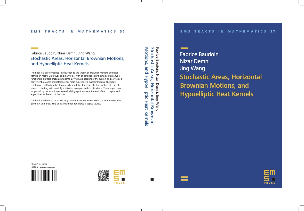
My new book written in collaboration with Nizar Demni and Jing Wang is now available.

This book is a self-contained introduction to the theory of Brownian motions and heat kernels on matrix Lie groups and manifolds, with an emphasis on the study of area type functionals. It offers graduate students a systematic account of the subject and serves as a convenient resource and reference for more experienced mathematicians. The book emphasizes methods rather than results and takes the reader to the frontiers of current research, starting with carefully motivated examples and constructions. These aspects are supported by the inclusion of several bibliographic notes at the end of each chapter and appendices at the end of the book.

This book can be used as a self-study guide for readers interested in the interplay between geometry and probability or as a textbook for a special topics course.

A preliminary version is available here.

Posted in Uncategorized | Leave a comment

Lecture 25, Einstein manifolds

Further topics, part 2

Lecture 25, Further topics
Posted in Einstein manifolds | Leave a comment

Lecture 24, Einstein manifolds

Further topics

Lecture 24
Posted in Einstein manifolds | Leave a comment

Lecture 23, Einstein manifolds

In this lecture we prove that quaternion Kahler manifolds are Einstein.

Lecture 23, Quaternion-Kahler
Posted in Einstein manifolds | Leave a comment

Lecture 22, Einstein manifolds

In this lecture, we keep going over the Calabi-Yau theorem and start speaking about quaternion Kahler manifolds.

Lecture 22, Calabi-Yau
Posted in Einstein manifolds | Leave a comment

Lecture 21, Ricci form and Calabi-Yau theorem

Lecture 21
Posted in Einstein manifolds | Leave a comment