Research and Lecture notes

Lecture 20. The Brownian motion as a rough path (1)

Posted on January 28, 2013 by Fabrice Baudoin

It is now time to give a fundamental example of rough path: The Brownian motion. As we are going to see, a Brownian motion is a $p$ -rough path for any $2 < p < 3$ .

We first remind the following basic definition.
Definition: Let $(\Omega,\mathcal{F},\mathbb{P})$ be a probability space. A continuous $d$ -dimensional process $(B_t)_{t \ge 0}$ is called a standard Brownian motion if it is a Gaussian process with mean function
$m(t)=0$
and covariance function
$R(s,t)=\mathbb{E}(B_s \otimes B_t)=\min (s,t) \mathbf{I}_d.$

For a Brownian motion $(B_t)_{t \ge 0}$ , the following properties are easy to check:

$B_0=0$ a.s.;
For any $h \geq 0$ , the process $(B_{t+h} - B_h)_{t \ge 0}$ is a standard Brownian motion;
For any $t > s\geq 0$ , the random variable $B_t -B_s$ is independent of the $\sigma$ -algebra $\sigma(B_u, u \le s )$ .
For every $c > 0$ , the process $(B_{ct})_{t \geq 0}$ has the same law as the process $(\sqrt{c} B_t)_{t \geq 0}$ .

An easy computation shows that for $n \ge 0$ and $0 \le s \le t$ :
$\mathbb{E} \left( \|B_t - B_s\|^{2n} \right)=\frac{(2n)!}{2^n n!} (t-s)^n.$
Therefore, as a consequence of the Kolmogorov continuity theorem, for any $T \ge 0$ and $0 \le \varepsilon < 1/2$ , there exists a finite random variable $C_{T, \varepsilon}$ such that for $0 \le s \le t \le T$ ,
$\| B_t -B_s \| \le C_{T, \varepsilon} |t-s|^{1/2-\varepsilon }.$
We deduce in particular that for any $p > 2$ , we have almost surely
$\| B\|_{p-var,[0,T]} < +\infty.$

We now prove that for $1 \le p < 2$ , we have almost surely
$\| B\|_{p-var,[0,T]}=+\infty.$

In the sequel, if
$\Delta_n [0,t]=\left\{ 0=t^n_0 \le t^n_1 \le ...\le t^n_n=t \right\}$
is a subdivision of the time interval $[0,t]$ , we denote by
$\mid\Delta_n [0,t] \mid=\max \{ \mid t^n_{k+1}-t^n_k \mid , k=0,...,n-1 \},$
the mesh of this subdivision.

Proposition: Let $(B_t)_{t\ge 0}$ be a standard Brownian motion. Let $t \ge 0$ . For every sequence $\Delta_n [0,t]$ of subdivisions such that
$\lim_{n \rightarrow +\infty}\mid\Delta_n [0,t]\mid=0,$
the following convergence takes place in $L^2$ (and thus in probability),
$\lim_{n \rightarrow +\infty} \sum_{k=1}^{n} \left\| B_{t^n_k}-B_{t^n_{k-1}}\right\|^2=t.$
As a consequence, if $1 \le p < 2$ , for every $T \ge 0$ , almost surely,
$\| B\|_{p-var,[0,T]}=+\infty.$

Proof: We prove the result in dimension 1 and let the reader adapt it to the multidimensional setting.
Let us denote
$V_n=\sum_{k=1}^{n} \left( B_{t^n_k} -B_{t^n_{k-1}}\right)^2.$
Thanks to the stationarity and the independence of Brownian increments, we have:
$\mathbb{E} \left( (V_n-t)^2\right)=\mathbb{E} \left( V_n^2\right)-2t\mathbb{E} \left( V_n\right)+t^2$
$=\sum_{j,k=1}^n\mathbb{E} \left( \left( B_{t^n_j} -B_{t^n_{j-1}}\right)^2\left( B_{t^n_k} -B_{t^n_{k-1}}\right)^2\right)-t^2$
$=\sum_{k=1}^n\mathbb{E} \left( \left( B_{t^n_j} -B_{t^n_{j-1}}\right)^4\right)+2\sum_{1\le j<k\le n}^n\mathbb{E} \left( \left( B_{t^n_j} -B_{t^n_{j-1}}\right)^2\left( B_{t^n_k} -B_{t^n_{k-1}}\right)^2\right)-t^2$
$=\sum_{k=1}^n (t^n_k-t^n_{k-1})^2 \mathbb{E} \left( B_1^4\right)+2\sum_{1\le j<k\le n}^n (t^n_j-t^n_{j-1})(t^n_k-t^n_{k-1})-t^2$
$=3\sum_{k=1}^n (t^n_j-t^n_{j-1})^2+2\sum_{1\le j<k\le n}^n (t^n_j-t^n_{j-1})(t^n_k-t^n_{k-1})-t^2$
$=2\sum_{k=1}^n (t^n_k-t^n_{k-1})^2$
$\le 2t\mid\Delta_n [0,t]\mid \rightarrow_{n \rightarrow +\infty} 0.$

Let us now prove that, as a consequence of this convergence, the paths of the process $(B_t)_{t\ge 0}$ almost surely have an infinite $p$ -variation on the time interval $[0,t]$ if $1 \le p < 2$ . Reasoning by absurd, let us assume that $\| B \|_{p-var,[0,t]} \le M$ . From the above result, since the convergence in probability implies the existence of an almost surely convergent subsequence, we can find a sequence of subdivisions $\Delta_n [0,t]$ whose mesh tends to $0$ and such that almost surely,
$\lim_{n \rightarrow +\infty} \sum_{k=1}^{n} \left( B_{t^n_k}-B_{t^n_{k-1}}\right)^2=t.$
We get then
$\sum_{k=1}^{n} \left( B_{t^n_k} -B_{t^n_{k-1}}\right)^2 \le M^p \sup_{1\le k \le n} \mid B_{t^n_k} -B_{t^n_{k-1}} \mid^{2-p} \rightarrow_{n \rightarrow +\infty} 0,$
which is clearly absurd $\square$

Therefore only the case $p=2$ is let open. It is actually possible to prove that:

Proposition: For every $T \ge 0$ , we have almost surely
$\| B \|_{2-var,[0,T]} = +\infty.$

Proof: See the book by Friz-Victoir page 381 $\square$

Posted in Rough paths theory | Leave a comment

Lecture 19. Geometric rough paths

Posted on January 27, 2013 by Fabrice Baudoin

In this Lecture, the geometric concepts introduced in the previous lectures are now used to revisit the notion of $p$ -rough path that was introduced before. We will see that using Carnot groups gives a perfect description of the space of $p$ -rough paths through the notion of geometric rough path.

Definition: Let $p \ge 1$ . An element $x \in C_0^{p-var} ([0,T], \mathbb{G}_{[p]} (\mathbb{R}^d))$ is called a geometric $p$ -rough path if there exists a sequence $x_n \in C_0^{1-var} ([0,T], \mathbb{G}_{[p]} (\mathbb{R}^d))$ that converges to $x$ in the $p$ -variation distance. The space of geometric $p$ -rough paths will be denoted by $\mathbf{\Omega G}^p([0,T],\mathbb{R}^d)$ .

To have it in mind, we recall the definition of a $p$ -rough path.

Definition: Let $p \ge 1$ and $x \in C_0^{p-var}([0,T],\mathbb{R}^d)$ . We say that $x$ is a $p$ -rough path if there exists a sequence $x_n \in C_0^{1-var}([0,T],\mathbb{R}^d)$ such that $x_n\to x$ in $p$ -variation and such that for every $\varepsilon > 0$ , there exists $N \ge 0$ such that for $m,n \ge N$ ,
$\sum_{j=1}^{[p]} \left\| \int dx_n^{\otimes j}- \int dx_m^{\otimes j} \right\|^{1/j}_{\frac{p}{j}-var, [0,T]} \le \varepsilon.$
The space of $p$ -rough paths is denoted $\mathbf{\Omega}^p([0,T],\mathbb{R}^d)$ .

Our first goal is of course to relate the notion of geometric rough path to the notion of rough path.

Proposition: Let $y \in C_0^{p-var} ([0,T], \mathbb{G}_{[p]} (\mathbb{R}^d))$ be a geometric $p$ -rough path, then the projection of $y$ onto $\mathbb{R}^d$ is a $p$ -rough path.

Proof: Let $y \in C_0^{p-var} ([0,T], \mathbb{G}_{[p]} (\mathbb{R}^d))$ be a geometric $p$ -rough path and let us consider a sequence $y_n \in C_0^{1-var} ([0,T], \mathbb{G}_{[p]} (\mathbb{R}^d))$ that converges to $y$ in the $p$ -variation distance. Denote by $x$ the projection of $y$ onto $\mathbb{R}^d$ and by $x_n$ the projection of $y_n$ . From a previous theorem $y_n=S_{[p]}(x_n)$ . It is clear that $x_n$ converges to $x$ in $p$ -variation. So, we want to prove that for every $\varepsilon > 0$ , there exists $N \ge 0$ such that for $m,n \ge N$ ,
$\sum_{j=1}^{[p]} \left\| \int dx_n^{\otimes j}- \int dx_m^{\otimes j} \right\|^{1/j}_{\frac{p}{j}-var, [0,T]} \le \varepsilon.$
Let us now keep in mind that
$d_{p-var; [s,t]}(y_n,y_m)=\left(\sup_{ \Pi \in \mathcal{D}[s,t]} \sum_{k=0}^{n-1} d( y_n(t_k)^{-1}y_n(t_{k+1}) , y_m(t_k)^{-1}y_m(t_{k+1}))^{p}\right)^{1/p}.$
and consider the control
$\omega(s,t)=\left( \frac{ d_{p-var; [s,t]}(y_n,y_m)}{d_{p-var; [0,T]}(y_n,y_m) } \right)^p+\left( \frac{ d_{p-var; [s,t]}(0,y_m)}{d_{p-var; [0,T]}(0,y_m) } \right)^p.$
We have
$\left\| \int dx_n^{\otimes k}- \int dx_m^{\otimes k} \right\|_{\frac{p}{k}-var, [0,T]}$
$= \left(\sup_{ \Pi \in \mathcal{D}[0,T]} \sum_{j=0}^{n-1} \left\| \int_{\Delta^k [t_j,t_{j+1}]} dx_n^{\otimes k}- \int _{\Delta^k [t_j,t_{j+1}]} dx_m^{\otimes k} \right\|^{p/k}\right)^{k/p}$
$\le \left( \sup_{0 \le s \le t \le T} \frac{ \left\| \int_{\Delta^k [s,t]} dx_n^{\otimes k}- \int _{\Delta^k [s,t]} dx_m^{\otimes k} \right\|}{\omega(s,t)^{k/p} } \right) \omega(0,T)^{k/p}$
From the ball-box estimate, there is a constant $C$ such that for $x,y \in \mathbb{G}_{[p]}(\mathbb{R}^d)$ :
$\| x-y \| \le C \max \{ d(x,y) \max \{ 1, d(0,x)^{N-1} \}, d(x,y)^N \}.$
We deduce
$\frac{ \left\| \int_{\Delta^k [s,t]} dx_n^{\otimes k}- \int _{\Delta^k [s,t]} dx_m^{\otimes k} \right\|}{\omega(s,t)^{k/p} }$
$\le C \max \left\{ d_{p-var; [0,T]}(y_n,y_m) \max \{ 1, d_{p-var; [0,T]}(0,y_m)^{N-1} \}, d_{p-var; [0,T]}(y_n,y_m)^N \right\}$
and thus
$\left\| \int dx_n^{\otimes k}- \int dx_m^{\otimes k} \right\|_{\frac{p}{k}-var, [0,T]} \le C' d_{p-var; [0,T]}(y_n,y_m)$
This is the estimate we were looking for $\square$

Conversely, any $p$ -rough path admits at least one lift as a geometric $p$ -rough path.

Proposition: Let $x \in C_0^{p-var} ([0,T], \mathbb{R}^d)$ be a $p$ -rough path. There exists a geometric $p$ -rough path $y \in \mathbf{\Omega G}^p([0,T],\mathbb{R}^d)$ such that the projection of $y$ onto $\mathbb{R}^d$ is $x$ .

Proof: Consider a sequence $x_n \in C_0^{1-var}([0,T],\mathbb{R}^d)$ such that $x_n\to x$ in $p$ -variation and such that for every $\varepsilon > 0$ , there exists $N \ge 0$ such that for $m,n \ge N$ ,
$\sum_{j=1}^{[p]} \left\| \int dx_n^{\otimes j}- \int dx_m^{\otimes j} \right\|^{1/j}_{\frac{p}{j}-var, [0,T]} \le \varepsilon.$
We claim that $y_n=S_{[p]} (x_n)$ is a sequence that converges in $p$ -variation to some $y \in \mathbf{\Omega G}^p([0,T],\mathbb{R}^d)$ such that the projection of $y$ onto $\mathbb{R}^d$ is $x$ . Let us consider the control
$\omega(s,t)= \left(\frac{ \sum_{j=1}^{[p]} \left\| \int dx_n^{\otimes j}- \int dx_m^{\otimes j} \right\|^{1/j}_{\frac{p}{j}-var, [s,t]}} { \sum_{j=1}^{[p]} \left\| \int dx_n^{\otimes j}- \int dx_m^{\otimes j} \right\|^{1/j}_{\frac{p}{j}-var, [0,T]}} \right)^p+\left( \frac{ d_{p-var; [s,t]}(0,y_m)}{d_{p-var; [0,T]}(0,y_m) } \right)^p.$
We have
$d_{p-var; [0,T]}(y_n,y_m) \le \left( \sup_{0 \le s \le t \le T} \frac{ d \left( y_n(s)^{-1}y_n(t), y_m(s)^{-1}y_m(t) \right) }{\omega(s,t)^{1/p} } \right) \omega(0,T)^{1/p}$
and argue as above to get, thanks to the ball-box theorem, an estimate like
$d_{p-var; [0,T]}(y_n,y_m) \le C \left( \sum_{j=1}^{[p]} \left\| \int dx_n^{\otimes j}- \int dx_m^{\otimes j} \right\|^{1/j}_{\frac{p}{j}-var, [0,T]}\right)^{1/N}$
$\square$

In general, we stress that there may be several geometric rough paths with the same projection onto $\mathbb{R}^d$ . The following proposition is useful to prove that a given path is a geometric rough path.

Proposition: If $q < p$ , then $C_0^{q-var} ([0,T], \mathbb{G}_{[p]} (\mathbb{R}^d)) \subset \mathbf{\Omega G}^p([0,T],\mathbb{R}^d)$ .

Proof: As in Euclidean case, it is not difficult to prove that $x \in \mathbf{\Omega G}^p([0,T],\mathbb{R}^d)$ if and only if
$\lim_{\delta \to 0} \sup_{ \Pi \in \Delta[s,t], | \Pi | \le \delta } \sum_{k=0}^{n-1} d( x(t_k), x(t_{k+1}) )^p=0,$
which is easy to check when $x \in C_0^{q-var} ([0,T], \mathbb{G}_{[p]} (\mathbb{R}^d))$ $\square$

If $y \in \mathbf{\Omega G}^p([0,T],\mathbb{R}^d)$ , then as we just saw, the projection $x$ of $y$ onto $\mathbb{R}^d$ is a $p$ -rough path and we can write
$y(t)=1+\sum_{k=1}^{[p]} \int_{\Delta^k[0,t]} dx^{\otimes k}.$
This is a convenient way to write geometric rough paths that we will often use in the sequel. For $N \ge [p]$ we can then define the lift of $y$ in $\mathbf{\Omega G}^N([0,T],\mathbb{R}^d)$ as:
$S_N(y)(t) =1+\sum_{k=1}^{N} \int_{\Delta^k[0,t]} dx^{\otimes k}.$
The following result is then easy to prove by using the previous results.

Proposition: Let $p \ge 1$ and $N \ge [p]$ . There exist constants $C_1,C_2 > 0$ such that for every $y \in \mathbf{\Omega G}^p([0,T],\mathbb{R}^d)$ ,
$\| y \|_{p-var,[0,T]} \le \| S_{N} (y) \|_{p-var; [0,T]} \le C_2 \| y \|_{p-var,[0,T]}.$

Posted in Rough paths theory | Leave a comment

Lecture 18. Paths with bounded p-variation in Carnot groups

Posted on January 14, 2013 by Fabrice Baudoin

In this Lecture, we go one step further to understand $p$ -rough paths from paths in Carnot groups. The connection is made through the study of paths with bounded p-variation in Carnot groups.

Definition: A continuous path $x : [s,t] \to \mathbb{G}_N(\mathbb{R}^d)$ is said to have a bounded variation on $[s,t]$ , if the 1-variation of $x$ on $[s,t]$ , which is defined as
$\| x \|_{1-var; [s,t]} :=\sup_{ \Pi \in \mathcal{D}[s,t]} \sum_{k=0}^{n-1} d( x(t_{k+1}) , x(t_k)),$
is finite, where $d$ is the Carnot-Caratheodory distance on $\mathbb{G}_N(\mathbb{R}^d)$ . The space of continuous bounded variation paths $x : [s,t] \to \mathbb{R}^d$ , will be denoted by $C^{1-var} ([s,t], \mathbb{G}_N(\mathbb{R}^d))$ .

The 1-variation distance between $x,y \in C^{1-var} ([s,t], \mathbb{G}_N(\mathbb{R}^d))$ is then defined as
$d_{1-var; [s,t]}=\sup_{ \Pi \in \mathcal{D}[s,t]} \sum_{k=0}^{n-1} d( x(t_k)^{-1}x(t_{k+1}), y(t_k)^{-1}y(t_{k+1})).$

As for the linear case the following proposition is easy to prove:

Proposition: Let $x \in C^{1-var} ([0,T], \mathbb{G}_N(\mathbb{R}^d))$ . The function $(s,t)\to \| x \|_{1-var, [s,t]}$ is additive, i.e for $0 \le s \le t \le u \le T$ ,
$\| x \|_{1-var, [s,t]}+ \| x \|_{1-var, [t,u]}= \| x \|_{1-var, [s,u]},$
and controls $x$ in the sense that for $0 \le s \le t \le T$ ,
$d(x(s),x(t))\le \| x \|_{1-var, [s,t]}.$
The function $s \to \| x \|_{1-var, [0,s]}$ is moreover continuous and non decreasing.

We will denote $C_0^{1-var} ([0,T], \mathbb{G}_N(\mathbb{R}^d)$ the space of continuous bounded variation paths that start at 0. It turns out that $C_0^{1-var} ([0,T], \mathbb{G}_N(\mathbb{R}^d))$ is always isometric to $C_0^{1-var} ([0,T], \mathbb{R}^d)$ . Remember that for $x \in C^{1-var} ([0,T], \mathbb{R}^d)$ , the lift of $x$ in $\mathbb{G}_N(\mathbb{R}^d)$ is denoted by $S_N(x)$ .

Definition: For every, $x \in C_0^{1-var} ([0,T], \mathbb{R}^d)$ , we have
$\| S_N(x) \|_{1-var; [0,T]}=\| x \|_{1-var; [0,T]}.$
Moreover, for every $y \in C_0^{1-var} ([0,T], \mathbb{G}_N(\mathbb{R}^d)$ , there exists one and only one $x \in C_0^{1-var} ([0,T], \mathbb{R}^d)$ such that $y=S_N(x).$

Proof: Let $x \in C_0^{1-var} ([0,T], \mathbb{R}^d)$ . From the very definition of the Carnot-Caratheodory distance, for $0 \le s \le t \le T$ , we have
$d(S_N(x)(s),S_N(x)(t)) \ge \| x \|_{1-var, [s,t]}.$
As a consequence we obtain,
$\| S_N(x) \|_{1-var; [0,T]} \ge \| x \|_{1-var; [0,T]}.$
On the other hand, $S_N(x)$ is the solution of the differential equation
$S_N(x)(t)=\sum_{i=1}^d \int_0^t X_i( S_N(x)(s)) dx^i(s), \quad 0 \le t \le T.$
This implies,
$d\left(S_N(x)(s), S_N(x)(t)\right) \le \int_s^t \| dx(u)\|= \| x \|_{1-var, [s,t]}.$
Finally, let $y \in C_0^{1-var} ([0,T], \mathbb{G}_N(\mathbb{R}^d)$ . Let $x$ be the projection of $y$ onto $\mathbb{R}^d$ . From the theorem of equivalence of homogeneous norms, we deduce that $x$ has a bounded variation in $\mathbb{R}^d$ . We claim that $y=S_N(x)$ . Consider the path $z=y S_N(x)^{-1}$ . This is a bounded variation path whose projection on $\mathbb{R}^d$ is 0. We want to prove that it implies that $z=0$ . Denote by $z_2$ the projection of $z$ onto $\mathbb{G}_2(\mathbb{R}^d)$ . Again from the equivalence of homogeneous norms, we see that $z_2$ has a bounded variation in $\mathbb{G}_2(\mathbb{R}^d)$ . Since the projection of $z_2$ on $\mathbb{R}^d$ is 0, we deduce that $z_2$ is in the center of $\mathbb{G}_2(\mathbb{R}^d)$ , which implies that $z_2(s)^{-1}z_2(t)=z_2(t)-z_2(s)$ . From the equivalence of homogeneous norms, we have then
$d(z_2(s),z_2(t)) \simeq \| z_2(t)-z_2(s) \|^{1/2}.$
Since $z_2$ has a bounded variation in $\mathbb{G}_2(\mathbb{R}^d)$ , it has thus a $1/2$ -variation for the Euclidean norm. This implies $z_2=0$ . Using the same argument inductively shows that for $n \le N$ , the projection of $z$ onto $\mathbb{G}_n(\mathbb{R}^d)$ will be 0. We conclude $z=0$ $\square$

As a conclusion, bounded variation paths in Carnot groups are the lifts of the bounded variation paths in $\mathbb{R}^d$ . As we will see, the situation is very different for paths with bounded $p$ -variation when $p \ge 2$ .

Definition: Let $p \ge 1$ . A continuous path $x : [s,t] \to \mathbb{G}_N(\mathbb{R}^d)$ is said to have a bounded $p$ -variation on $[s,t]$ , if the p-variation of $x$ on $[s,t]$ , which is defined as
$\| x \|_{p-var; [s,t]} :=\left( \sup_{ \Pi \in \mathcal{D}[s,t]} \sum_{k=0}^{n-1} d( x(t_{k+1}) , x(t_k))^p\right)^{1/p},$
is finite. The space of continuous paths $x : [s,t] \to \mathbb{R}^d$ with a $p$ -bounded variation will be denoted by $C^{p-var} ([s,t], \mathbb{G}_N(\mathbb{R}^d))$ .

The $p$ -variation distance between $x,y \in C^{p-var} ([s,t], \mathbb{G}_N(\mathbb{R}^d))$ is then defined as
$d_{p-var; [s,t]}=\left(\sup_{ \Pi \in \mathcal{D}[s,t]} \sum_{k=0}^{n-1} d( x(t_k)^{-1}x(t_{k+1}) , y(t_k)^{-1}y(t_{k+1}))^p\right)^{1/p}.$

As for $\mathbb{R}^d$ valued paths, we restrict our attention to $p \ge 1$ because any path with a $p$ -bounded variation, $p < 1$ needs to be constant. We have then the following theorem that extends the previous result. The proof is somehow similar to the previous result, so we let the reader fill the details.

Theorem: Let $1 \le p < 2$ . For every $y \in C_0^{p-var} ([0,T], \mathbb{G}_N(\mathbb{R}^d)$ , there exists one and only one $x \in C_0^{p-var} ([0,T], \mathbb{R}^d)$ such that
$y=S_N(x).$
Moreover, we have
$\| x \|_{p-var; [0,T]} \le \| S_N(x) \|_{p-var; [0,T]}\le C\| x \|_{p-var; [0,T]}.$

For $p \ge 2$ , the situation is different as we are going to explain in the next Lectures. This can already be understood by using the estimates on iterated integrals that were obtained in a previous Lecture. Indeed, we have the following very important proposition that already shows the connection between $p$ -rough paths and paths with a bounded $p$ -variation in Carnot groups:

Proposition: Let $p \ge 1$ and $N \ge [p]$ . There exist constants $C_1,C_2 > 0$ such that for every $x \in C_0^{1-var} ([0,T], \mathbb{G}_N(\mathbb{R}^d)$ ,
$C_1 \left( \sum_{j=1}^{[p]} \left\| \int dx^{\otimes j}\right\|^{1/j}_{\frac{p}{j}-var, [s,t]} \right) \le \| S_{N} (x) \|_{p-var; [s,t]} \le C_2 \left( \sum_{j=1}^{[p]} \left\| \int dx^{\otimes j}\right\|^{1/j}_{\frac{p}{j}-var, [s,t]} \right).$

Proof: This is a consequence of the theorem about the equivalence of homogeneous norms on Carnot groups. Write the stratification of $\mathfrak{g}_N(\mathbb{R}^d)$ as:
$\mathfrak{g}_N(\mathbb{R}^d)=\mathcal{V}_1 \oplus \cdots \oplus \mathcal{V}_N$
and denote by $\pi_i$ the projection onto $\mathcal{V}_i$ . Let us denote by $\| \cdot \|$ the norm on $\mathfrak{g}_N(\mathbb{R}^d)$ that comes from the norm on formal series. Then,
$\rho(g)=\sum_{i=1}^N \| \pi_i (g) \|^{1/i}$
is an homogeneous norm on $\mathbb{G}_N(\mathbb{R}^d)$ . Thus, there exist constants $C_1,C_2 > 0$ such that for every $g \in \mathbb{G}_N(\mathbb{R}^d)$ ,
$C_1 \rho(g) \le d(0,g) \le C_2 \rho (g).$
In particular, we get
$C_1 \rho\left(S_N(x)(s)^{-1}S_N(x)(t)\right) \le d\left(S_N(x)(s), S_N(x)(t)\right) \le C_2 \rho \left(S_N(x)(s)^{-1}S_N(x)(t)\right).$
Let us now observe that
$\rho\left( (S_N(x)(s))^{-1} S_N(x)(t) \right)=\sum_{k=1}^N \left\| \int_{\Delta^k [s,t]} dx^{\otimes k} \right\|^{1/k}$
and that, from a previous lecture $k \ge [p]$ ,
$\left\| \int_{\Delta^k [s,t]} dx^{\otimes k} \right\| \le \frac{C^k}{\left( \frac{k}{p}\right)!} \left( \sum_{j=1}^{[p]} \left\| \int dx^{\otimes j}\right\|^{1/j}_{\frac{p}{j}-var, [s,t]} \right)^k, \quad 0 \le s \le t \le T.$
The conclusion easily follows $\square$

Posted in Rough paths theory | Leave a comment

Lecture 17. The Carnot Carathéodory distance

Posted on January 7, 2013 by Fabrice Baudoin

In this Lecture we introduce a canonical distance on a Carnot group. This distance is naturally associated to the sub-Riemannian structure which is carried by a Carnot group. It plays a fundamental role in the rough paths topology. Let $\mathbb{G}_N(\mathbb{R}^d)$ be the free Carnot group over $\mathbb{R}^d$ . Remember that if $x \in C^{1-var}([0,T],\mathbb{R}^d)$ , then we denote by $S_N(x)$ the lift of $x$ in $\mathbb{G}_N(\mathbb{R}^d)$ . The first important concept is the notion of horizontal curve.

Definition: A curve $y: [0,1] \to \mathbb{G}_N(\mathbb{R}^d)$ is said to be horizontal if there exists $x \in C^{1-var}([0,T],\mathbb{R}^d)$ such that $y=S_N(x)$ .

It is remarkable that any two points of $\mathbb{G}_N(\mathbb{R}^d)$ can be connected by a horizontal curve.

Proposition: Given two points $g_1$ and $g_2 \in \mathbb{G}_N(\mathbb{R}^d)$ , there is at least one $x \in C^{1-var}([0,T],\mathbb{R}^d)$ such that $g_1S_N(x)(1)=g_2$ .

Proof: Let us denote by $G$ the subgroup of diffeomorphisms $\mathbb{G}_N(\mathbb{R}^d) \rightarrow \mathbb{G}_N(\mathbb{R}^d)$ generated by the one-parameter subgroups corresponding to $X_1, \cdots , X_d$ . The Lie algebra of $G$ can be identified with the Lie algebra generated by $X_1, \cdots , X_d$ , i.e. $\mathfrak{g}_N(\mathbb{R}^d)$ . We deduce that $G$ can be identified with $\mathbb{G}_N(\mathbb{R}^d)$ itself, so that it acts transitively on $\mathbb{G}$ . It means that for every $x \in \mathbb{G}_N(\mathbb{R}^d)$ , the map $G \rightarrow \mathbb{G}_N(\mathbb{R}^d)$ , $g \rightarrow g(x)$ is surjective. Thus, every two points in $\mathbb{G}$ can be joined by a piecewise smooth horizontal curve where each piece is a segment of an integral curve of one of the vector fields $\mathbf{e}_i$ $\square$

In the above proof, the horizontal curve constructed to join the two points is not smooth. Nevertheless, it can be shown that it is always possible to connect two points with a smooth horizontal curve.

Let us also remark that this theorem is a actually a very special case of the so-called Chow-Rashevski theorem which is one of the cornerstones of sub-Riemannian geometry. We now are ready for the definition of the Carnot-Carathéodory distance.

Definition For $g_1,g_2 \in \mathbb{G}_N(\mathbb{R}^d)$ , we define
$d(g_1,g_2)=\inf_{\mathcal{S}(g_1,g_2)} \| x \|_{1-var,[0,1]},$
where
$\mathcal{S}(g_1,g_2)=\{ x \in C^{1-var}([0,1],\mathbb{R}^d), g_1S_N(x)(1)=g_2 \}.$
$d(g_1,g_2)$ is called the Carnot-Carathéodory distance between $g_1$ and $g_2$ .

The first thing to prove is that $d$ is indeed a distance.
Lemma: The Carnot-Carathéodory distance is indeed a distance.

Proof: The symmetry and the triangle inequality are easy to check and we let the reader find the arguments. The last thing to prove is that $d(g_1,g_2)=0$ implies $g_1=g_2$ . From the definition of $d$ it clear that $d_R \le d$ where $d_R$ is the Riemmanian measure on $\mathbb{G}_N(\mathbb{R}^d)$ . It follows that $d(g_1,g_2)=0$ implies $g_1=g_2$ $\square$

We then observe the following properties of $d$ :

Proposition:

For $g_1,g_2 \in \mathbb{G}_N(\mathbb{R}^d)$ , $d(g_1,g_2)=d(g_2,g_1)=d(0,g_1^{-1} g_2).$

Let $(\Delta_t)_{t \ge 0}$ be the one parameter family of dilations on $\mathbb{G}_N(\mathbb{R}^d)$ . For $g_1,g_2 \in \mathbb{G}_N(\mathbb{R}^d)$ , and $t \ge 0$ , $d(\Delta_t g_1,\Delta_t g_2)=t d(g_1,g_2)$ .

Proof: The first part of the proposition stems from the fact that for every $x \in C^{1-var}([0,T],\mathbb{R}^d)$ , $S_N(x)^{-1}= S_N(-x)$ , so that $g_1S_N(x)(1)=g_2$ is equivalent to $g_2S_N(-x)(1)=g_1$ which also equivalent to $S_N(x)(1)=g_1^{-1} g_2$ . For the second part, we observe that for $t \ge 0$ , $\Delta_t S_N(x)=S_N(tx)$ $\square$

The Carnot-Carathéodory distance is pretty difficult to explicitly compute in general. It is often much more convenient to estimate using a so-called homogeneous norm.

Definition: A homogeneous norm on $\mathbb{G}_N(\mathbb{R}^d)$ is a continuous function $\parallel \cdot \parallel : \mathbb{G}_N(\mathbb{R}^d) \rightarrow [0,+\infty)$ , such that:

$\parallel \Delta_t x \parallel=t \parallel x \parallel$ , $t \ge 0$ , $x \in \mathbb{G}_N(\mathbb{R}^d)$ ;

$\parallel x^{-1} \parallel= \parallel x \parallel$ , $x \in \mathbb{G}_N(\mathbb{R}^d)$ ;

$\parallel x \parallel=0$ if and only if $x=0$ .

It turns out that the Carnot-Carathéodory distance is equivalent to any homogeneous norm in the following sense:

Theorem: Let $\parallel \cdot \parallel$ be a homogeneous norm on $\mathbb{G}_N(\mathbb{R}^d)$ . There exist two positive constants $C_1$ and $C_2$ such that for every $x,y \in \mathbb{G}_N(\mathbb{R}^d)$ ,
$A \| x^{-1}y \| \le d(x,y) \le B \| x^{-1}y \|.$

By using the left invariance of $d$ , it is of course enough to prove that for every $x \in \mathbb{G}_N(\mathbb{R}^d)$ ,
$A \| x \| \le d(0,x) \le B \| x \|.$
We first prove that the function $x\to d(0,x)$ is bounded on compact sets (of the Riemannian topology of the Lie group $\mathbb{G}_N(\mathbb{R}^d)$ ). As we have seen before, every $x \in \mathbb{G}_N(\mathbb{R}^d)$ can be written as a product:
$x=\prod_{i=1}^N e^{t_i X_{k_i}}.$
From the very definition of the distance, we have then
$d(0,x)\le d\left(0,\prod_{i=1}^N e^{t_i X_{k_i}}\right)\le \sum_{i=1}^N |t_i|.$
It is not difficult to see that $\sum_{i=1}^N |t_i|$ can uniformly be bounded on compact sets, therefore $d(0,x)$ is bounded on compact sets. Consider now the compact set
$\mathbf{K}= \{ x \in \mathbb{G}_N(\mathbb{R}^d), \| x \|=1 \}.$
Since $d(0,x)$ is bounded on $K$ , we deduce that there exists a constant $B$ such that for every $x \in \mathbf{K}$ ,
$d(0,x) \le B.$
Since $d_R \le d$ , where $d_R$ is the Riemannian distance, we deduce that there exists a constant $A$ such that for every $x \in \mathbf{K}$ ,
$d(0,x) \ge A.$
Now, for every $x \in \mathbb{G}_N(\mathbb{R}^d)$ , $x \neq 0$ , we deduce that
$A \le d\left( 0, \Delta_{1/\| x \|} x \right) \le B$
This yields the expected result $\square$

Let us give an example of a homogeneous norm which is particularly adapted to rough paths theory. Write the stratification of $\mathfrak{g}_N(\mathbb{R}^d)$ as:
$\mathfrak{g}_N(\mathbb{R}^d)=\mathcal{V}_1 \oplus \cdots \oplus \mathcal{V}_N$ and denote by $\pi_i$ the projection onto $\mathcal{V}_i$ . Let us denote by $\| \cdot \|$ the norm on $\mathfrak{g}_N(\mathbb{R}^d)$ that comes from the norm on formal series. Then, it is easily checked that
$\rho(g)=\sum_{i=1}^N \| \pi_i (g) \|^{1/i}$
is an homogeneous norm on $\mathbb{G}_N(\mathbb{R}^d)$ . This homogeneous norm is particulary adapted to the study of paths because if $x \in C^{1-var}([0,T], \mathbb{R}^d)$ , then one has:
$\rho\left( (S_N(x)(s))^{-1} S_N(x)(t) \right)=\sum_{k=1}^N \left\| \int_{\Delta^k [s,t]} dx^{\otimes k} \right\|^{1/k}$

We finally quote the following result, not difficult to prove which is often referred to as the ball-box estimate.

Proposition: There exists a constant $C$ such that for every $x,y \in \mathbb{G}_N(\mathbb{R}^d)$ ,
$d(x,y) \le C \max \{ \| x-y \|, \| x -y \|^{1/N} \max \{ 1, d(0,x)^{1-1/N} \} \}.$
and
$\| x-y \| \le C \max \{ d(x,y) \max \{ 1, d(0,x)^{N-1} \}, d(x,y)^N \}.$
In particular, for every compact set $K \subset \mathbb{G}_N(\mathbb{R}^d)$ , there is a constant $C_K$ such that for every $x,y \in K$ ,
$\frac{1}{C_K} \| x-y\| \le d(x,y) \le C_K \| x -y \|^{1/N}.$

Proof: See the book by Friz-Victoir, page 152 $\square$

Posted in Rough paths theory | Leave a comment

Lecture 16. Free Carnot groups

Posted on January 5, 2013 by Fabrice Baudoin

We introduce here the notion of Carnot group, which is the correct structure to understand the algebra of the iterated integrals of a path up to a given order. It is worth mentioning that these groups play a fundamental role in sub-Riemannian geometry as they appear as the tangent cones to sub-Riemannian manifolds.

Definition: A Carnot group of step (or depth) $N$ is a simply connected Lie group $\mathbb{G}$ whose Lie algebra can be written
$\mathcal{V}_{1}\oplus...\oplus \mathcal{V}_{N},$
with
$\lbrack \mathcal{V}_{i},\mathcal{V}_{j}]=\mathcal{V}_{i+j}$
and $\mathcal{V}_{s}=0,\text{ for }s > N.$

There are some basic examples of Carnot groups.

Example 1: The group $\left( \mathbb{R}^d ,+ \right)$ is the only commutative Carnot group.

Example 2: (Heisenberg group) Consider the set $\mathbb{H}_n =\mathbb{R}^{2n} \times \mathbb{R}$ endowed with the group law
$(x,\alpha) \star (y, \beta)=\left( x+y, \alpha + \beta +\frac{1}{2} \omega (x,y) \right),$
where $\omega$ is the standard symplectic form on $\mathbb{R}^{2n}$ , that is
$\omega(x,y)= x^t \left( \begin{array}{ll} 0 & -\mathbf{I}_{n} \\ \mathbf{I}_{n} & ~~~0 \end{array} \right) y.$
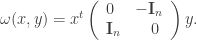
On $\mathfrak{h}_n$ the Lie bracket is given by
$[ (x,\alpha) , (y, \beta) ]=\left( 0, \omega (x,y) \right),$
and it is easily seen that $\mathfrak{h}_n=\mathcal{V}_1 \oplus \mathcal{V}_2,$ where $\mathcal{V}_1 =\mathbb{R}^{2n} \times \{ 0 \}$ and $\mathcal{V}_2= \{ 0 \} \times \mathbb{R}$ . Therefore $\mathbb{H}_n$ is a Carnot group of depth 2.

The Carnot group $\mathbb{G}$ is said to be free if $\mathfrak{g}$ is isomorphic to the nilpotent free Lie algebra with $d$ generators. In that case, $\dim \mathcal{V}_{j}$ is the number of Hall words of length $j$ in the free algebra with $d$ generators. A combinatorial argument shows then that:
$\dim \mathcal{V}_{j}= \frac{1}{j} \sum_{i \mid j} \mu (i) d^{\frac{j}{i}}, \text{ } j \leq N,$
where $\mu$ is the Möbius function. A consequence from this is that when $N \rightarrow +\infty$ ,
$\dim \mathfrak{g} \sim \frac{d^N}{N}.$
The free Carnot groups are the ones that will be the most relevant for us, so from now on, we will restrict our attention to them.

Let $\mathbb{G}$ be a free Carnot group of step $N$ . Notice that the vector space $\mathcal{V}_{1}$ , which is called the basis of $\mathbb{G}$ , Lie generates $\mathfrak{g}$ , where $\mathfrak{g}$ denotes the Lie algebra of $\mathbb{G}$ . Since $\mathbb{G}$ is step $N$ nilpotent and simply connected, the exponential map is a diffeomorphism and the Baker-Campbell-Hausdorff formula therefore completely characterizes the group law of $\mathbb{G}$ because for $U,V \in \mathfrak{g}$ ,
$\exp U \exp V = \exp \left( P (U,V) \right)$
for some universal Lie polynomial $P$ whose first terms are given by
$P (U,V) = U+V+\frac{1}{2} [U,V] +\frac{1}{12} [[U,V],V]-\frac{1}{12}[[U,V],U]$
$-\frac{1}{48} [V,[U,[U,V]]]-\frac{1}{48} [U,[V,[U,V]]]+\cdots.$
On $\mathfrak{g}$ we can consider the family of linear operators $\delta_{t}:\mathfrak{g} \rightarrow \mathfrak{g}$ , $t \geq 0$ which act by scalar multiplication $t^{i}$ on $\mathcal{V}_{i}$ . These operators are Lie algebra automorphisms due to the grading. The maps $\delta_t$ induce Lie group automorphisms $\Delta_t :\mathbb{G} \rightarrow \mathbb{G}$ which are called the canonical dilations of $\mathbb{G}$ .

It is an interesting fact that every free Carnot group of step $N$ is isomorphic to some $\mathbb{R}^m$ endowed with a polynomial group law. Indeed, let $X_1,\cdots,X_d$ be a basis of $\mathcal{V}_{1}$ . From the Hall-Witt theorem we can construct a basis of $\mathfrak{g}$ which is adapted to the grading
$\mathfrak{g}=\mathcal{V}_{1}\oplus \cdots \oplus \mathcal{V}_{N},$
and such that every element of this basis is an iterated bracket of the $X_i$ ‘s. Such basis, which can be made quite explicit, will be referred to as a Hall basis over $X_1,\cdots,X_d$ . Let $\mathcal{B}$ be such a basis. For $X \in \mathfrak{g}$ , let $[X]_\mathcal{B}$ be the coordinate vector of $X$ in the basis $\mathcal{B}$ . If we denote by $m$ the dimension of $\mathfrak{g}$ , we see that we can define a group law $\star$ on $\mathbb{R}^m$ by the requirement that for $X,Y \in \mathfrak{g}$ ,
$[X]_\mathcal{B} \star [Y]_\mathcal{B} =[ P_N(X,Y) ]_\mathcal{B}=[ \ln (e^X e^Y) ]_\mathcal{B}.$
It is then clear that $(\mathbb{R}^m, \star)$ is a Carnot group of step $N$ whose Lie bracket is given by:
$[ [X]_\mathcal{B} , [Y]_\mathcal{B}] =[ [X,Y] ]_\mathcal{B}.$
Therefore, every free Carnot group of step $N$ such that $\dim \mathcal{V}_{1}=d$ is isomorphic to $(\mathbb{R}^m, \star)$ . Another representation of the free Carnot group of step $N$ which is particularly adapted to rough paths theory is given in the framework of formal series. As before, let us denote by $\mathbb{R}[[X_1, \cdots, X_d ]]$ the set formal series. Let us denote by $\mathbb{R}_N[X_1,\cdots,X_d]$ the set of truncated series at order $N$ , that is $\mathbb{R}[[X_1, \cdots, X_d ]]$ quotiented by $X_{i_1}\cdots X_{i_k}=0$ if $k \ge N+1$ . In this context, the free nilpotent Lie algebra of order $N$ can be identified with the Lie algebra generated by $X_1,\cdots,X_d$ inside $\mathbb{R}_N[X_1,\cdots,X_d]$ , where the bracket is of course given by the anticommutator. This representation of the free nilpotent Lie algebra of depth $N$ shall be denoted by $\mathfrak{g}_N(\mathbb{R}^d)$ in the sequel of the course. The free nilpotent group of step can then be represented as $\mathbb{G}_N(\mathbb{R}^d)=\exp ( \mathfrak{g}_N(\mathbb{R}^d))$ where the exponential map is the usual exponential of formal series.

We are now ready for the definition of the lift of a path in $\mathbb{G}_N(\mathbb{R}^d)$ .

Definition: Let $x \in C^{1-var}([0,T],\mathbb{R}^d)$ . The $\mathbb{G}_N(\mathbb{R}^d)$ valued path
$\sum_{k=0}^{N} \int_{\Delta^k [0,t]} dx^{\otimes k}, \quad 0 \le t \le T,$
is called the lift of $x$ in $\mathbb{G}_N(\mathbb{R}^d)$ and will be denoted by $S_N(x)$ .

It is worth noticing that $S_N(x)$ is indeed valued in $\mathbb{G}_N(\mathbb{R}^d)$ because from the Chen’s expansion formula:
$S_N(x)(t)=\exp \left( \sum_{k = 1}^N \sum_{I \in \{1,\cdots ,d\}^k}\Lambda_I (x)_{t} X_I \right),$
where the notations have been introduced before. The multiplicativity property of the signature also immediately implies that for $s \le t$ ,
$S_N(x)(t)=S_N(x)(s)\exp\left( \sum_{k = 1}^N \sum_{I \in \{1,\cdots ,d\}^k}\Lambda_I (x)_{s,t} X_I\right).$

Posted in Rough paths theory | Leave a comment

Lecture 15. The Magnus expansion

Posted on January 3, 2013 by Fabrice Baudoin

In the previous lecture, we proved the Chen’s expansion formula which establishes the fact that the signature of a path is the exponential of a Lie series. This expansion is of course formal but analytically makes sense in a number of situations that we now describe. The first case of study are linear equations.

Let us consider matrices $M_1,\cdots,M_d \in \mathbb{R}^{n \times n}$ and let $y_n:[0,T] \to \mathbb{R}^n$ be the solution of the differential equation
$y(t)=y(0)+\sum_{i=1}^d \int_0^t M_i y(s)d x^i(s),$
where $x \in C^{1-var}([0,T],\mathbb{R}^d)$ . The solution $y$ admits a representation as an absolutely convergent Volterra series
$y(t)=y(0)+ \sum^{+\infty}_{k=1}\sum_{I=(i_1,\cdots,i_k)} M_{i_1}\cdots M_{i_k} \left( \int_{\Delta^{k}[0,t]}dx^{I} \right) y(0).$
The formal analogy between this expansion and the signature leads to the following result:

Proposition: There exists $\tau > 0$ such that for $0 \le t \le \tau$ ,
$y(t)= \exp \left( \sum_{k \geq 1} \sum_{I \in \{1,\cdots ,d\}^k}\Lambda_I (x)_{t} M_I \right)y(0),$
where
$M_I = [M_{i_1},[M_{i_2},...,[M_{i_{k-1}}, M_{i_{k}}]...],$
is the iterated Lie bracket and
$\Lambda_I (x)_{t}= \sum_{\sigma \in \mathcal{S}_k} \frac{\left(-1\right) ^{e(\sigma )}}{k^{2}\left( \begin{array}{l} k-1 \\ e(\sigma ) \end{array} \right) } \int_{\Delta^k[0,t]} dx^{\sigma^{-1} \cdot I}.$

Proof: We only give the sketch of the proof. Details can be found in this paper by Strichartz. First, we observe that a combinatorial argument shows that
$\sum_{\sigma \in \mathcal{S}_k} \frac{1}{\left( \begin{array}{l} k-1 \\ e(\sigma ) \end{array} \right) } \le \frac{C}{2^k} k! \sqrt{k}.$
On the other hand, we have the estimate
$\left| \int_{\Delta^k[0,t]} dx^{\sigma^{-1} \cdot I} \right| \le \int_{\Delta^k[0,t]} \| dx^{\sigma^{-1} \cdot I}\| \le \frac{1}{k!} \| x \|^k_{1-var, [0,t]}.$
As a consequence, we obtain
$\left| \Lambda_I (x)_{t} \right| \le \frac{C}{2^k k^{3/2}} \| x \|^k_{1-var, [0,t]}.$
For the matrix norm we have the estimate $\| M_I \| \le C^k,$ so we conclude that for some constant $\tilde{C}$ ,
$\left\| \sum_{I \in \{1,\cdots ,d\}^k}\Lambda_I (x)_{t} M_I \right\| \le \frac{\tilde{C}^k}{ k^{3/2}} \| x \|^k_{1-var, [0,t]}.$
We deduce that if $\tau$ is such that $\| x \|_{1-var, [0,\tau]} < \frac{1}{\tilde{C}}$ , then the series
$\sum_{k \geq 1} \sum_{I \in \{1,\cdots ,d\}^k}\Lambda_I (x)_{t} M_I$
is absolutely convergent on the interval $[0,\tau]$ . At this point, we can observe that the Chen's expansion formula is a purely algebraic statement, thus expanding the exponential
$\exp\left( \sum_{k \geq 1} \sum_{I \in \{1,\cdots ,d\}^k}\Lambda_I (x)_{t} M_I \right)y(0)$
and rearranging the terms leads to
$y(0)+ \sum^{+\infty}_{k=1}\sum_{I=(i_1,\cdots,i_k)} M_{i_1}\cdots M_{i_k} \left( \int_{\Delta^{k}[0,t]}dx^{I} \right) y(0)$
which is equal to $y(t)$ $\square$

Another framework, close to this linear case, in which the Chen's expansion makes sense are Lie groups. Let $\mathbb{G}$ be a Lie group acting on $\mathbb{R}^d$ . Let us denote by $\mathfrak{g}$ the Lie algebra of $\mathbb{G}$ . Elements of $\mathfrak{g}$ can be seen as vector fields on $\mathbb{R}^d$ . Indeed, for $X\in \mathfrak{g}$ , we can define
$X(x)=\lim_{t \to 0} \frac{ e^{tX}(x)-x}{t},$
where $e^{tX}$ is the exponential mapping on the Lie group $\mathbb{G}$ . With this identification, it is easily checked that the Lie bracket in the Lie algebra coincides with the Lie bracket of vector fields and that the exponential map $e^{tX}$ in the group corresponds to the flow generated by the vector field $X$ . As above we get then the following result:

Proposition: Let $V_1,\cdots, V_d \in \mathfrak{g}$ and $x \in C^{1-var}([0,T], \mathbb{R}^d)$ . Let us consider the differential equation
$y(t)=y(0)+\sum_{i=1}^d \int_0^t V_i(y(s)) dx^i(s).$
There exists $\tau > 0$ such that for $0 \le t \le \tau$ ,
$y(t)= \exp \left( \sum_{k \geq 1} \sum_{I \in \{1,\cdots ,d\}^k}\Lambda_I (x)_{t} V_I \right)y(0).$

A special case will be of interest for us: The case where the Lie group $\mathbb{G}$ is nilpotent. Let us recall that a Lie group $\mathbb{G}$ is said to be nilpotent of order $N$ if every bracket of length greater or equal to $N+1$ is 0. In that case, the sum in the exponential is finite and the representation is then of course valid on the whole time interval $[0,T]$ .

Posted in Rough paths theory | Leave a comment

Lecture 14. The Chen expansion formula

Posted on January 2, 2013 by Fabrice Baudoin

The next few lectures will be devoted to the construction of the so-called geometric rough paths. These paths are the lifts of the $p$ -rough paths in the free nilpotent Lie group of order $p$ . The construction which is of algebraic and geometric nature will give a clear understanding and description of the space of rough paths. The starting point of the geometric rough path construction is the algebraic study of the signature. We present first the results for continuous paths with bounded variation because the extension to $p$ -rough paths is more or less trivial.

Let us first remind that if $x \in C^{1-var}([0,T],\mathbb{R}^d)$ , then the signature of $x$ is defined as the formal series
$\mathfrak{S} (x)_{s,t}$
$=1 + \sum_{k=1}^{+\infty} \sum_{I \in \{1,...,d\}^k} \left( \int_{s \leq t_1 \leq ... \leq t_k \leq t} dx^{i_1}_{t_1} \cdots dx^{i_k}_{t_k} \right) X_{i_1} \cdots X_{i_k}$
$=1+\sum_{k=1}^{+\infty} \int_{\Delta^k[0,T]} dx^{\otimes k}.$

If the indeterminates $X_1,\cdots,X_d$ commute (that is if we work in the commutative algebra of formal series), then the signature of a path admits a very nice representation.

Indeed, let us denote by $\mathcal{S}_k$ the group of the permutations of the index set $\{1,...,k\}$ and if $\sigma \in \mathcal{S}_k$ , we denote for a word $I=(i_1,...,i_k)$ , $\sigma \cdot I$ the word $(i_{\sigma(1)},...,i_{\sigma(k)})$ . By commuting $X_1,\cdots,X_d$ we get
$\mathfrak{S} (x)_{s,t} = 1+ \sum_{k=1}^{+\infty} \sum_{I=(i_1,...,i_k)} X_{i_1} ... X_{i_k} \left( \frac{1}{k!} \sum_{\sigma \in \mathcal{S}_k} \int_{\Delta^k [s,t]} dx^{\sigma \cdot I} \right).$
Since
$\sum_{\sigma \in \mathcal{S}_k} \int_{\Delta^k [s,t]} dx^{\sigma \cdot I} =(x^{i_1}(t)-x^{i_1}(s)) \cdots (x^{i_k}(t)-x^{i_k}(s)),$
we deduce,
$\mathfrak{S} (x)_t$
$= 1+ \sum_{k=1}^{+\infty} \frac{1}{k!} \sum_{I=(i_1,...,i_k)} X_{i_1} \cdots X_{i_k}(x^{i_1}(t)-x^{i_1}(s)) \cdots (x^{i_k}(t)-x^{i_k}(s))$
$=\exp \left( \sum_{i=1}^d (x^i(t)-x^i(s)) X_i \right)$
where the exponential of a formal series $Y$ is, of course, defined as
$\exp (Y)=\sum_{k=0}^{+\infty} \frac{Y^k}{k!}.$
As a consequence, the commutative signature of a path is simply the exponential of the increments of the path. Of course, the formula is only true in the commutative case. In the general and non-commuting case, it is remarkable that there exists a nice formula that expresses the signature as the exponential of a quite explicit series which turns out to be a Lie series (a notion defined below). We need to introduce first a few notations.

We define the Lie bracket between two elements $U$ and $V$ of $\mathbb{R} [[ X_1 ,\cdots , X_d ]]$ by $[U,V]=UV-VU$ . Moreover, if $I=(i_1,...,i_k) \in \{ 1,\cdots , d \}^k$ is a word, we denote by $X_I$ the iterated Lie bracket which is defined by
$X_I = [X_{i_1},[X_{i_2},...,[X_{i_{k-1}}, X_{i_{k}}]...].$

Theorem: If $x \in C^{1-var}([0,T],\mathbb{R}^d)$ , then
$\mathfrak{S} (x)_{s,t} =\exp \left( \sum_{k \geq 1} \sum_{I \in \{1,\cdots ,d\}^k}\Lambda_I (x)_{s,t} X_I \right), \text{ } 0 \le s \le t \le T,$
where for $k \ge 1, \text{ }I \in \{1,\cdots ,d\}^k$ :

$\mathcal{S}_k$ is the set of the permutations of $\{1,\cdots ,k\}$ ;

If $\sigma \in \mathcal{S}_k$ , $e(\sigma)$ is the cardinality of the set
$\{ j \in \{1,\cdots ,k-1 \} , \sigma (j) > \sigma(j+1) \},$

$\Lambda_I (x)_{s,t}= \sum_{\sigma \in \mathcal{S}_k} \frac{\left(-1\right) ^{e(\sigma )}}{k^{2}\left( \begin{array}{l} k-1 \\ e(\sigma ) \end{array} \right) } \int_{\Delta^k[s,t]} dx^{\sigma^{-1} \cdot I}.$

The first terms in the formula are:
$\sum_{I=(i_1)} \Lambda_I (x)_{s,t} X_I=\sum_{k=1}^d (x^i(t)-x^i(s)) X_i$
and
$\sum_{I=(i_1,i_2)} \Lambda_I (x)_{s,t} X_I=\frac{1}{2} \sum_{1 \leq i<j \leq d} [X_i , X_j] \int_s^t x^i(u) dx^j(u) - x^j(u) dx^i(u).$

The proof proceeds in several steps. To simplify a little the notations we will assume $s=0$ , $t=T$ and $x(0)=0$ . The idea is to prove first the result when the path $x$ is piecewise linear that is
$x(t)=x(t_i)+ a_i (t-t_i)$
on the interval $[t_i,t_{i+1})$ where $0=t_0\le t_1 \le \cdots \le t_N =T$ . And, then, we will use a limiting argument.

The key point here is the multiplicativity property for the signature that already was pointed out in a previous lecture: For $0\le s \le t \le u \le T$ ,
$\mathfrak{S} (x)_{s,u}=\mathfrak{S} (x)_{s,t}\mathfrak{S} (x)_{t,u}.$
By using inductively the multiplicative property, we obtain
$\mathfrak{S} (x)_{0,T}=\prod_{n=0}^{N-1} \left( \mathbf{1} + \sum_{k=1}^{+\infty} \sum_{I=(i_1,...i_k)} X_{i_1} ... X_{i_k} \int_{\Delta^k [t_n,t_{n+1}]} dx^I \right)$

Since, on $[t_n,t_{n+1})$ ,
$dx(t)=a_n dt,$
we have
$\int_{\Delta^k [t_n,t_{n+1}]} dx^I =a_n^{i_1} \cdots a_n^{i_k} \int_{\Delta^k [t_n,t_{n+1}]} dt_{i_1} \cdots dt_{i_k} =a_n^{i_1} \cdots a_n^{i_k} \frac{(t_{n+1}-t_n)^k}{k!}.$
Therefore
$\mathfrak{S} (x)_{0,T}$
$=\prod_{n=0}^{N-1} \left( \mathbf{1} + \sum_{k=1}^{+\infty} \sum_{I=(i_1,...i_k)} X_{i_1} ... X_{i_k} a_n^{i_1} \cdots a_n^{i_k} \frac{(t_{n+1}-t_n)^k}{k!} \right)$
$=\prod_{n=0}^{N-1} \exp \left( (t_{n+1}-t_n) \sum_{i=0}^d a_n^i X_i \right).$

We now use the Baker-Campbell-Hausdorff-Dynkin formula that gives a quite explicit formula for the product of exponentials of non commuting variables:

Proposition: If $y_1,\cdots,y_N \in \mathbb{R}^{d}$ then,
$\prod_{n=1}^{N}\exp \left( \sum_{i=1}^d y_n^i X_i \right) =\exp \left( \sum_{k \geq 1} \sum_{I \in \{1,...,d\}^k}\beta_I (y_1,\cdots,y_N) X_I \right),$
where for $k \ge 1, \text{ }I \in \{1,...,d\}^k$ :
$\beta_I (y_1,\cdots,y_N) =\sum_{\sigma \in \mathcal{S}_k} \sum_{1=j_0 \le j_1 \le \cdots \le j_{N-1} \le k} \frac{\left(-1\right) ^{e(\sigma )}}{j_1!\cdots j_{N-1}! k^{2}\left( \begin{array}{l} k-1 \\ e(\sigma ) \end{array} \right) } \prod_{\nu=1}^{N} y_\nu^{\sigma^{-1}(i_{j_{\nu-1}+1})} \cdots y_\nu^{\sigma^{-1}(i_{j_\nu})}$ .

We get therefore:
$\mathfrak{S} (x)_{0,T}=\exp \left( \sum_{k \geq 1} \sum_{I \in \{1,...,d\}^k}\beta_I (t_1 a_0,\cdots,(t_N-t_{N-1})a_{N-1}) X_I \right).$
It is finally an exercise to check, by using the Chen relations, that:
$\beta_I (t_1 a_0,\cdots,(t_N-t_{N-1})a_{N-1})= \sum_{\sigma \in \mathcal{S}_k} \frac{\left(-1\right) ^{e(\sigma )}}{k^{2}\left( \begin{array}{l} k-1 \\ e(\sigma ) \end{array} \right) } \int_{\Delta^k[0,T]} dx^{\sigma^{-1} \cdot I}.$

We conclude that if $x$ is piecewise linear then the formula
$\mathfrak{S} (x)_{s,t} =\exp \left( \sum_{k \geq 1} \sum_{I \in \{1,\cdots ,d\}^k}\Lambda_I (x)_{s,t} X_I \right), \text{ } 0 \le s \le t \le T$

holds. Finally, if $x \in C^{1-var}([0,T],\mathbb{R}^d)$ , then we can consider the sequence $x_n$ of linear interpolations along a subdivision of $[0,T]$ whose mesh goes to 0. For this sequence, all the iterated integrals $\int_{\Delta^k[0,T]} dx_n^{ I}$ will converge to $\int_{\Delta^k[0,T]} dx^{ I}$ (see for instance the proposition 2.7 in the book by Friz-Victoir) and the result follows.

Posted in Rough paths theory | Leave a comment

Lecture 13. Linear differential equations driven by rough paths

Posted on January 2, 2013 by Fabrice Baudoin

In this lecture we define solutions of linear differential equations driven by $p$ -rough paths, $p \ge 1$ and present the Lyons’ continuity theorem in this setting. Let $x \in \mathbf{\Omega}^p([0,T],\mathbb{R}^d)$ be a $p$ -rough path with truncated signature $\sum_{k=0}^{[p]} \int_{\Delta^k [s,t]} dx^{\otimes k},$ and let $x_n \in C^{1-var}([0,T],\mathbb{R}^d)$ be an approximating sequence such that
$\sum_{j=1}^{[p]} \left\| \int dx^{\otimes j}- \int dx_n^{\otimes j} \right\|^{1/j}_{\frac{p}{j}-var, [0,T]} \to 0.$

Let us consider matrices $M_1,\cdots,M_d \in \mathbb{R}^{n \times n}$ . We have the following theorem:

Theorem: Let $y_n:[0,T] \to \mathbb{R}^n$ be the solution of the differential equation
$y_n(t)=y(0)+\sum_{i=1}^d \int_0^t M_i y_n(s)d x^i_n(s).$
Then, when $n \to \infty$ , $y_n$ converges in the $p$ -variation distance to some $y \in C^{p-var}([0,T],\mathbb{R}^n)$ . $y$ is called the solution of the rough differential equation
$y(t)=y(0)+\sum_{i=1}^d \int_0^t M_i y(s)d x^i(s).$

Proof: It is a classical result that the solution of the equation
$y_n(t)=y(0)+\sum_{i=1}^d \int_0^t M_i y_n(s)d x^i_n(s),$
can be expanded as the convergent Volterra series:
$y_n(t)=y_n(s)+ \sum^{+\infty}_{k=1}\sum_{I=(i_1,\cdots,i_k)} M_{i_1}\cdots M_{i_k} \left( \int_{\Delta^{k}[s,t]}dx_n^{I} \right) y_n(s).$
Therefore, in particular, for $n,m \ge 0$ ,
$y_n(t)-y_p(t)=\sum^{+\infty}_{k=1}\sum_{I=(i_1,\cdots,i_k)} M_{i_1}\cdots M_{i_k} \left( \int_{\Delta^{k}[0,t]}dx_n^{I}- \int_{\Delta^{k}[0,t]}dx_p^{I} \right) y(0),$
which implies that
$\| y_n(t)-y_m(t) \| \le \sum^{+\infty}_{k=1}M^k \left\| \int_{\Delta^{k}[0,t]}dx_n^{\otimes k}- \int_{\Delta^{k}[0,t]}dx_m^{\otimes k} \right\| \| y(0) \|$
with $M=\max \{ \| M_1 \| , \cdots , \| M_d \| \}$ . From the theorems of the previous lectures, there exists a constant $C \ge 0$ depending only on $p$ and
$\sup_n \sum_{j=1}^{[p]} \left\| \int dx_n^{\otimes j} \right\|^{1/j}_{\frac{p}{j}-var, [0,T]}$
such that for $k \ge 1$ and $n,m$ big enough:
$\left\| \int_{\Delta^k [0,\cdot]} dx_n^{\otimes k}- \int_{\Delta^k [0,\cdot]} dx_m^{\otimes k} \right\|_{p-var, [0,T]} \le \left( \sum_{j=1}^{[p]} \left\| \int dx_n^{\otimes j}- \int dx_m^{\otimes j} \right\|^{1/j}_{\frac{p}{j}-var, [0,T]} \right) \frac{C^k}{\left( \frac{k}{p}\right)!}.$
As a consequence, there exists a constant $\tilde{C}$ such that for $n,m$ big enough:
$\| y_n(t)-y_m(t) \| \le \tilde{C} \sum_{j=1}^{[p]} \left\| \int dx_n^{\otimes j}- \int dx_m^{\otimes j} \right\|^{1/j}_{\frac{p}{j}-var, [0,T]} .$
This already proves that $y_n$ converges in the supremum topology to some $y$ . We now have
$(y_n(t)-y_n(s))-(y_m(t)-y_m(s))$
$=\sum^{+\infty}_{k=1}\sum_{I=(i_1,\cdots,i_k)} M_{i_1}\cdots M_{i_k} \left( \int_{\Delta^{k}[s,t]}dx_n^{I}y_n(s) -\int_{\Delta^{k}[s,t]}dx_m^{I} y_m(s)\right),$
and we can bound
$\left\| \int_{\Delta^{k}[s,t]}dx_n^{I}y_n(s) -\int_{\Delta^{k}[s,t]}dx_m^{I} y_m(s) \right\|$
$\le \left\| \int_{\Delta^{k}[s,t]}dx_n^{I} \right\| \| y_n(s)-y_m(s) \|+\| y_m(s) \| \left\| \int_{\Delta^{k}[s,t]}dx_n^{I} - \int_{\Delta^{k}[s,t]}dx_m^{I}\right\|$
$\le \left\| \int_{\Delta^{k}[s,t]}dx_n^{I} \right\| \| y_n-y_m \|_{\infty, [0,T]} +\| y_m \|_{\infty, [0,T]} \left\| \int_{\Delta^{k}[s,t]}dx_n^{I} - \int_{\Delta^{k}[s,t]}dx_m^{I}\right\|$
Again, from the theorems of the previous lectures, there exists a constant $C \ge 0$ , depending only on $p$ and
$\sup_n \sum_{j=1}^{[p]} \left\| \int dx_n^{\otimes j} \right\|^{1/j}_{\frac{p}{j}-var, [0,T]}$
such that for $k \ge 1$ and $n,m$ big enough
$\left\| \int_{\Delta^k [s,t]} dx_n^{\otimes k} \right\| \le \frac{C^k}{\left( \frac{k}{p}\right)!} \omega(s,t)^{k/p}, \quad 0 \le s \le t \le T.$
$\left\| \int_{\Delta^k [s,t]} dx_n^{\otimes k}- \int_{\Delta^k [s,t]} dx_m^{\otimes k} \right\| \le \left( \sum_{j=1}^{[p]} \left\| \int dx_n^{\otimes j}- \int dx_m^{\otimes k} \right\|^{1/j}_{\frac{p}{j}-var, [0,T]} \right) \frac{C^k}{\left( \frac{k}{p}\right)!} \omega(s,t)^{k/p} ,$
where $\omega$ is a control such that $\omega(0,T)=1$ . Consequently, there is a constant $\tilde{C}$ , such that
$\| (y_n(t)-y_n(s))-(y_m(t)-y_m(s)) \|$
$\le \tilde{C} \left( \| y_n-y_m \|_{\infty, [0,T]} + \sum_{j=1}^{[p]} \left\| \int dx_n^{\otimes j}- \int dx_m^{\otimes k} \right\|^{1/j}_{\frac{p}{j}-var, [0,T]} \right) \omega(s,t)^{1/p}$
This implies the estimate
$\| y_n -y_m \|_{p-var,[0,T]} \le \tilde{C} \left( \| y_n-y_m \|_{\infty, [0,T]} + \sum_{j=1}^{[p]} \left\| \int dx_n^{\otimes j}- \int dx_m^{\otimes k} \right\|^{1/j}_{\frac{p}{j}-var, [0,T]} \right)$
and thus gives the conclusion $\square$

With just a little more work, it is possible to prove the following stronger result whose proof is let to the reader.
Theorem: Let $y_n:[0,T] \to \mathbb{R}^n$ be the solution of the differential equation
$y_n(t)=y(0)+\sum_{i=1}^d \int_0^t M_i y_n(s)d x^i_n(s).$
and $y$ be the solution of the rough differential equation:
$y(t)=y(0)+\sum_{i=1}^d \int_0^t M_i y(s)d x^i(s).$
Then, $y \in \mathbf{\Omega}^p([0,T],\mathbb{R}^d)$ and when $n \to \infty$ ,
$\sum_{j=1}^{[p]} \left\| \int dy^{\otimes j}- \int dy_n^{\otimes j} \right\|^{1/j}_{\frac{p}{j}-var, [0,T]} \to 0.$

We can get useful estimates for solutions of rough differential equations. For that, we need the following analysis lemma:

Proposition: For $x \ge 0$ and $p \ge 1$ ,
$\sum_{k=0}^{+\infty} \frac{x^k}{\left( \frac{k}{p} \right)!} \le p e^{x^p}.$

Proof: For $\alpha \ge 0$ , we denote
$E_\alpha(x)=\sum_{k=0}^{+\infty} \frac{x^k}{\left( k \alpha \right)!}.$
This is a special function called the Mittag-Leffler function. From the binomial inequality
$E_\alpha(x)^2$
$=\sum_{k=0}^{+\infty} \left( \sum_{j=0}^k \frac{1}{\left( j \alpha \right)!\left( (k-j) \alpha \right)!}\right)x^k$
$\le \frac{1}{\alpha}\sum_{k=0}^{+\infty} 2^{\alpha k} \frac{x^k}{\left( k \alpha \right)!}=\frac{1}{\alpha}E_\alpha(2^\alpha x).$
Thus we proved
$E_\alpha(x)\le\frac{1}{\alpha^{1/2}}E_\alpha(2^\alpha x)^{1/2}.$
Iterating this inequality, $k$ times we obtain
$E_\alpha(x)\le \frac{1}{\alpha^{\sum_{j=1}^k \frac{1}{2^j}}} E_\alpha(2^{\alpha k}x)^{1/(2k)}.$
It is known (and not difficult to prove) that
$E_\alpha(x) \sim_{x \to \infty} \frac{1}{\alpha} e^{x^{1/\alpha}}.$
By letting $k \to \infty$ we conclude
$E_\alpha(x) \le \frac{1}{\alpha} e^{x^{1/\alpha}}.$
$\square$

This estimate provides the following result:

Proposition: Let $y$ be the solution of the rough differential equation:
$y(t)=y(0)+\sum_{i=1}^d \int_0^t M_i y(s)d x^i(s).$
Then, there exists a constant $C$ depending only on $p$ such that for $0 \le t \le T$ ,
$\| y(t) \| \le p \| y(0)\| e^{ CM \left( \sum_{j=1}^{[p]} \left\| \int dx^{\otimes j} \right\|^{1/j}_{\frac{p}{j}-var, [0,t]} \right)^p},$
where $M=\max \{ \| M_1 \|, \cdots, \|M_d\| \}$ .

Proof: We have
$y(t)=y(0)+ \sum^{+\infty}_{k=1}\sum_{I=(i_1,\cdots,i_k)} M_{i_1}\cdots M_{i_k} \left( \int_{\Delta^{k}[0,t]}dx^{I} \right) y(0).$
Thus we obtain
$y(t)\le \left( 1+ \sum^{+\infty}_{k=1}\sum_{I=(i_1,\cdots,i_k)} M^k \left\| \int_{\Delta^{k}[0,t]}dx^{I} \right\| \right) \| y(0) \|$ ,
and we conclude by using estimates on iterated integrals of rough paths together with the previous lemma $\square$

Posted in Rough paths theory | Leave a comment

Lecture 12. p-rough paths

Posted on January 1, 2013 by Fabrice Baudoin

In this lecture, it is now time to harvest the fruits of the two previous lectures. This will allow us to finally define the notion of $p$ -rough path and to construct the signature of such path.

A first result which is a consequence of the theorem proved in the previous lecture is the following continuity of the iterated iterated integrals with respect to a convenient topology. The proof uses very similar arguments to the previous two lectures, so we let it as an exercise to the student.

This continuity result naturally leads to the following definition.

Definition: Let $p \ge 1$ and $x \in C^{p-var}([0,T],\mathbb{R}^d)$ . We say that $x$ is a $p$ -rough path if there exists a sequence $x_n \in C^{1-var}([0,T],\mathbb{R}^d)$ such that $x_n\to x$ in $p$ -variation and such that for every $\varepsilon > 0$ , there exists $N \ge 0$ such that for $m,n \ge N$ ,
$\sum_{j=1}^{[p]} \left\| \int dx_n^{\otimes j}- \int dx_m^{\otimes j} \right\|^{1/j}_{\frac{p}{j}-var, [0,T]} \le \varepsilon.$
The space of $p$ -rough paths will be denoted $\mathbf{\Omega}^p([0,T],\mathbb{R}^d)$ .

From the very definition, $\mathbf{\Omega}^p([0,T],\mathbb{R}^d)$ is the closure of $C^{1-var}([0,T],\mathbb{R}^d)$ inside $C^{p-var}([0,T],\mathbb{R}^d)$ for the distance
$d_{\mathbf{\Omega}^p([0,T],\mathbb{R}^d)}(x,y)= \sum_{j=1}^{[p]} \left\| \int dx^{\otimes j}- \int dy^{\otimes j} \right\|^{1/j}_{\frac{p}{j}-var, [0,T]} .$

If $x \in \mathbf{\Omega}^p([0,T],\mathbb{R}^d)$ and $x_n \in C^{1-var}([0,T],\mathbb{R}^d)$ is such that $x_n\to x$ in $p$ -variation and such that for every $\varepsilon > 0$ , there exists $N \ge 0$ such that for $m,n \ge N$ ,
$\sum_{j=1}^{[p]} \left\| \int dx_n^{\otimes j}- \int dx_m^{\otimes j} \right\|^{1/j}_{\frac{p}{j}-var, [0,T]} \le \varepsilon,$
then we define $\int_{\Delta^k [s,t]} dx^{\otimes k}$ for $k \le p$ as the limit of the iterated integrals $\int_{\Delta^k [s,t]} dx_n^{\otimes k}$ . However it is important to observe that $\int_{\Delta^k [s,t]} dx^{\otimes k}$ may then depend on the choice of the approximating sequence $x_n$ . Once the integrals $\int_{\Delta^k [s,t]} dx^{\otimes k}$ are defined for $k \le p$ , we can then use the previous theorem to construct all the iterated integrals $\int_{\Delta^k [s,t]} dx^{\otimes k}$ for $k > p$ . It is then obvious that if $x,y \in \mathbf{\Omega}^p([0,T],\mathbb{R}^d)$ , then
$1 + \sum_{k=1}^{[p]} \int_{\Delta^k [s,t]} dx^{\otimes k}=1 + \sum_{k=1}^{[p]} \int_{\Delta^k [s,t]} dy^{\otimes k}$
implies that
$1 + \sum_{k=1}^{+\infty } \int_{\Delta^k [s,t]} dx^{\otimes k}=1 + \sum_{k=1}^{+\infty} \int_{\Delta^k [s,t]} dy^{\otimes k}.$
In other words the signature of a $p$ -rough path is completely determinated by its truncated signature at order $[p]$ :
$\mathfrak{S}_{[p]} (x)_{s,t} =1 + \sum_{k=1}^{[p]} \int_{\Delta^k [s,t]} dx^{\otimes k}.$
For this reason, it is natural to present a $p$ -rough path by this truncated signature at order $[p]$ in order to stress that the choice of the approximating sequence to contruct the iterated integrals up to order $[p]$ has been made. This will be further explained in much more details when we will introduce the notion of geometric rough path over a rough path.

The following results are straightforward to obtain from the previous lectures by a limiting argument.

Lemma: Let $x \in \mathbf{\Omega}^p([0,T],\mathbb{R}^d)$ , $p \ge 1$ . For $0 \le s \le t \le u \le T$ , and $n \ge 1$ ,
$\int_{\Delta^n [s,u]} dx^{\otimes n}=\sum_{k=0}^{n} \int_{\Delta^k [s,t]} dx^{\otimes k }\int_{\Delta^{n-k} [t,u]} dx^{\otimes (n-k) }.$

Theorem: Let $p \ge 1$ . There exists a constant $C \ge 0$ , depending only on $p$ , such that for every $x \in\mathbf{\Omega}^p([0,T],\mathbb{R}^d)$ and $k \ge 1$ ,
$\left\| \int_{\Delta^k [s,t]} dx^{\otimes k} \right\| \le \frac{C^k}{\left( \frac{k}{p}\right)!} \left( \sum_{j=1}^{[p]} \left\| \int dx^{\otimes j}\right\|^{1/j}_{\frac{p}{j}-var, [s,t]} \right)^k, \quad 0 \le s \le t \le T.$

If $p \ge 2$ , the space $\mathbf{\Omega}^p([0,T],\mathbb{R}^d)$ is not a priori a Banach space (it is not a linear space) but it is a complete metric space for the distance
$d_{\mathbf{\Omega}^p([0,T],\mathbb{R}^d)}(x,y)= \sum_{j=1}^{[p]} \left\| \int dx^{\otimes j}- \int dy^{\otimes j} \right\|^{1/j}_{\frac{p}{j}-var, [0,T]} .$
The structure of $\mathbf{\Omega}^p([0,T],\mathbb{R}^d)$ will be better understood in the next lectures, but let us remind that if $1 \le p < 2$ , then $\mathbf{\Omega}^p([0,T],\mathbb{R}^d)$ is the closure of $C^{1-var}([0,T],\mathbb{R}^d)$ inside $C^{p-var}([0,T],\mathbb{R}^d)$ for the variation distance it is therefore what we denoted $C^{0,p-var}([0,T],\mathbb{R}^d)$ . As a corollary we deduce

Proposition: Let $1 \le p < 2$ . Then $x \in \mathbf{\Omega}^p([0,T],\mathbb{R}^d)$ if and only if
$\lim_{\delta \to 0} \sup_{ \Pi \in \mathcal{D}[s,t], | \Pi | \le \delta } \sum_{k=0}^{n-1} \| x(t_{k+1}) -x(t_k) \|^p=0,$
where $\mathcal{D}[s,t]$ is the set of subdivisions of $[s,t]$ . In particular, for $p < q < 2$ ,
$C^{q-var}([0,T],\mathbb{R}^d) \subset \mathbf{\Omega}^p([0,T],\mathbb{R}^d).$

Posted in Rough paths theory | Leave a comment

Lecture 11. Estimating iterated integrals (Part 2)

Posted on December 31, 2012 by Fabrice Baudoin

Let $x \in C^{1-var}([0,T],\mathbb{R}^d)$ . Since
$\omega(s,t)=\left( \sum_{j=1}^{[p]} \left\| \int dx^{\otimes j}\right\|^{1/j}_{\frac{p}{j}-var, [s,t]} \right)^p$
is a control, the estimate
$\left\| \int_{\Delta^k [s,t]} dx^{\otimes k} \right\| \le \frac{C^k}{\left( \frac{k}{p}\right)!} \left( \sum_{j=1}^{[p]} \left\| \int dx^{\otimes j}\right\|^{1/j}_{\frac{p}{j}-var, [s,t]} \right)^k, \quad 0 \le s \le t \le T.$
easily implies that for $k > p$ ,
$\left\| \int dx^{\otimes k} \right\|_{1-var, [s,t]} \le \frac{C^k}{\left( \frac{k}{p}\right)!} \omega(s,t)^{k/p}.$
We stress that it does not imply a bound on the 1-variation of the path $t \to \int_{\Delta^k [0,t]} dx^{\otimes k}$ . What we can get for this path, are bounds in $p$ -variation:

Proposition: Let $p \ge 1$ . There exists a constant $C \ge 0$ , depending only on $p$ , such that for every $x \in C^{1-var}([0,T],\mathbb{R}^d)$ and $k \ge 0$ ,
$\left\| \int_{\Delta^k [0,\cdot]} dx^{\otimes k} \right\|_{p-var, [s,t]} \le \frac{C^k}{\left( \frac{k}{p}\right)!} \omega(s,t)^{1/p} \omega(0,T)^{\frac{k-1}{p}}$
where
$\omega(s,t)= \left( \sum_{j=1}^{[p]} \left\| \int dx^{\otimes j}\right\|^{1/j}_{\frac{p}{j}-var, [s,t]} \right)^p, \quad 0 \le s \le t \le T.$

Proof: This is an easy consequence of the Chen’s relations. Indeed,

$\left\| \int_{\Delta^k [0,t]} dx^{\otimes k} - \int_{\Delta^k [0,s]} dx^{\otimes k} \right\|$
$=\left\| \sum_{j=1}^k \int_{\Delta^j [s,t]} dx^{\otimes j} \int_{\Delta^{j-k} [0,s]} dx^{\otimes (k-j)} \right\|$
$\le \sum_{j=1}^k \left\| \int_{\Delta^j [s,t]} dx^{\otimes j} \right\| \left\| \int_{\Delta^{j-k} [0,s]} dx^{\otimes (k-j)} \right\|$
$\le C^k \sum_{j=1}^k \frac{1}{\left( \frac{j}{p}\right)!} \omega(s,t)^{j/p} \frac{1}{\left( \frac{k-j}{p}\right)!} \omega(s,t)^{(k-j)/p}$
$\le C^k \omega(s,t)^{1/p} \sum_{j=1}^k \frac{1}{\left( \frac{j}{p}\right)!} \omega(0,T)^{(j-1)/p} \frac{1}{\left( \frac{k-j}{p}\right)!} \omega(0,T)^{(k-j)/p}$
$\le C^k \omega(s,t)^{1/p} \omega(0,T)^{(k-1)/p}\sum_{j=1}^k \frac{1}{\left( \frac{j}{p}\right)!} \frac{1}{\left( \frac{k-j}{p}\right)!}.$
and we conclude with the binomial inequality $\square$

We are now ready for a second major estimate which is the key to define iterated integrals of a path with $p$ -bounded variation when $p \ge 2$ .

Theorem: Let $p \ge 1$ , $K > 0$ and $x,y \in C^{1-var}([0,T],\mathbb{R}^d)$ such that
$\sum_{j=1}^{[p]} \left\| \int dx^{\otimes j}- \int dy^{\otimes j} \right\|^{1/j}_{\frac{p}{j}-var, [0,T]} \le 1,$
and
$\left( \sum_{j=1}^{[p]} \left\| \int dx^{\otimes j}\right\|^{1/j}_{\frac{p}{j}-var, [0,T]} \right)^p+ \left( \sum_{j=1}^{[p]} \left\| \int dy^{\otimes j}\right\|^{1/j}_{\frac{p}{j}-var, [0,T]} \right)^p \le K.$
Then there exists a constant $C \ge 0$ depending only on $p$ and $K$ such that for $0\le s \le t \le T$ and $k \ge 1$
$\left\| \int_{\Delta^k [s,t]} dx^{\otimes k}- \int_{\Delta^k [s,t]} dy^{\otimes k} \right\| \le \left( \sum_{j=1}^{[p]} \left\| \int dx^{\otimes j}- \int dy^{\otimes j} \right\|^{1/j}_{\frac{p}{j}-var, [0,T]} \right) \frac{C^k}{\left( \frac{k}{p}\right)!} \omega(s,t)^{k/p} ,$
$\left\| \int_{\Delta^k [s,t]} dx^{\otimes k}\right\| +\left\| \int_{\Delta^k [s,t]} dy^{\otimes k} \right\| \le \frac{C^k}{\left( \frac{k}{p}\right)!} \omega(s,t)^{k/p}$
where $\omega$ is the control
$\omega(s,t)= \frac{ \left( \sum_{j=1}^{[p]} \left\| \int dx^{\otimes j}\right\|^{1/j}_{\frac{p}{j}-var, [s,t]} \right)^p+ \left( \sum_{j=1}^{[p]} \left\| \int dy^{\otimes j}\right\|^{1/j}_{\frac{p}{j}-var, [s,t]} \right)^p } { \left( \sum_{j=1}^{[p]} \left\| \int dx^{\otimes j}\right\|^{1/j}_{\frac{p}{j}-var, [0,T]} \right)^p+ \left( \sum_{j=1}^{[p]} \left\| \int dy^{\otimes j}\right\|^{1/j}_{\frac{p}{j}-var, [0,T]} \right)^p }$
$+\left( \frac{\sum_{j=1}^{[p]} \left\| \int dx^{\otimes j} - \int dy^{\otimes j}\right\|^{1/j}_{\frac{p}{j}-var, [s,t]} }{\sum_{j=1}^{[p]} \left\| \int dx^{\otimes j} - \int dy^{\otimes j}\right\|^{1/j}_{\frac{p}{j}-var, [0,T]} } \right)^p$

Proof: We prove by induction on $k$ that for some constants $C,\beta$ ,
$\left\| \int_{\Delta^k [s,t]} dx^{\otimes k}- \int_{\Delta^k [s,t]} dy^{\otimes k} \right\| \le \left( \sum_{j=1}^{[p]} \left\| \int dx^{\otimes j}- \int dy^{\otimes j} \right\|^{1/j}_{\frac{p}{j}-var, [0,T]} \right) \frac{C^k}{\beta \left( \frac{k}{p}\right)!} \omega(s,t)^{k/p},$
$\left\| \int_{\Delta^k [s,t]} dx^{\otimes k}\right\| +\left\| \int_{\Delta^k [s,t]} dy^{\otimes k} \right\| \le \frac{C^k}{\beta \left( \frac{k}{p}\right)!} \omega(s,t)^{k/p}$

For $k \le p$ , we trivially have
$\left\| \int_{\Delta^k [s,t]} dx^{\otimes k}- \int_{\Delta^k [s,t]} dy^{\otimes k} \right\|$ $\le \left( \sum_{j=1}^{[p]} \left\| \int dx^{\otimes j}- \int dy^{\otimes j} \right\|^{1/j}_{\frac{p}{j}-var, [0,T]} \right)^k \omega(s,t)^{k/p}$
$\le \left( \sum_{j=1}^{[p]} \left\| \int dx^{\otimes j}- \int dy^{\otimes j} \right\|^{1/j}_{\frac{p}{j}-var, [0,T]} \right) \omega(s,t)^{k/p}.$
and
$\left\| \int_{\Delta^k [s,t]} dx^{\otimes k}\right\| +\left\| \int_{\Delta^k [s,t]} dy^{\otimes k} \right\| \le K^{k/p} \omega(s,t)^{k/p}$ .
Not let us assume that the result is true for $0 \le j \le k$ with $k > p$ . Let
$\Gamma_{s,t}=\int_{\Delta^k [s,t]} dx^{\otimes (k+1)}- \int_{\Delta^k [s,t]} dy^{\otimes (k+1)}$
From the Chen’s relations, for $0 \le s \le t \le u \le T$ ,
$\Gamma_{s,u}= \Gamma_{s,t}+ \Gamma_{t,u}$
$+\sum_{j=1}^{k} \int_{\Delta^j [s,t]} dx^{\otimes j }\int_{\Delta^{k+1-j} [t,u]} dx^{\otimes (k+1-j) }-\sum_{j=1}^{k} \int_{\Delta^j [s,t]} dy^{\otimes j }\int_{\Delta^{k+1-j} [t,u]} dy^{\otimes (k+1-j) }.$
Therefore, from the binomial inequality
$\| \Gamma_{s,u}\|$
$\le \| \Gamma_{s,t} \| + \| \Gamma_{t,u} \| +\sum_{j=1}^{k} \left\| \int_{\Delta^j [s,t]} dx^{\otimes j }- \int_{\Delta^j [s,t]} dy^{\otimes j } \right\| \left\| \int_{\Delta^{k+1-j} [t,u]} dx^{\otimes (k+1-j) }\right\|$
$+\sum_{j=1}^{k} \left\| \int_{\Delta^{j} [s,t]} dy^{\otimes j }\right\| \left\| \int_{\Delta^{k+1-j} [t,u]} dx^{\otimes (k+1-j) }- \int_{\Delta^{k+1-j} [t,u]} dy^{\otimes (k+1-j) } \right\|$
$\le \| \Gamma_{s,t} \| + \| \Gamma_{t,u} \| +\frac{1}{\beta^2}\tilde{\omega}(0,T) \sum_{j=1}^{k} \frac{C^j}{\left( \frac{j}{p}\right)!} \omega(s,t)^{j/p} \frac{C^{k+1-j}}{\left( \frac{k+1-j}{p}\right)!} \omega(t,u)^{(k+1-j)/p}$
$+\frac{1}{\beta^2}\tilde{\omega}(0,T) \sum_{j=1}^{k} \frac{C^j}{\left( \frac{j}{p}\right)!} \omega(s,t)^{j/p} \frac{C^{k+1-j}}{\left( \frac{k+1-j}{p}\right)!} \omega(t,u)^{(k+1-j)/p}$
$\le \| \Gamma_{s,t} \| + \| \Gamma_{t,u} \| +\frac{2p}{\beta^2} \tilde{\omega}(0,T) C^{k+1} \frac{ \omega(s,u)^{(k+1)/p}}{\left( \frac{k+1}{p}\right)! }$
where
$\tilde{\omega}(0,T)=\sum_{j=1}^{[p]} \left\| \int dx^{\otimes j}- \int dy^{\otimes j} \right\|^{1/j}_{\frac{p}{j}-var, [0,T]} .$
We deduce
$\| \Gamma_{s,t} \| \le \frac{2p}{\beta^2(1-2^{1-\theta})} \tilde{\omega}(0,T) C^{k+1} \frac{ \omega(s,t)^{(k+1)/p}}{\left( \frac{k+1}{p}\right)! }$
with $\theta= \frac{k+1}{p}$ . A correct choice of $\beta$ finishes the induction argument $\square$