With Hongyi Chen, Li Chen and Søren Kjærsgaard, we have posted a new paper, Intermittency for the parabolic Anderson model on spaces with sub-Gaussian heat kernel estimates.

This is a sequel to our earlier work on bounded domains of recurrent metric measure spaces, where we assumed strong recurrence, $d_h<d_w$, and considered Dirichlet and Neumann boundary conditions. The new paper treats unbounded spaces and allows critical and transient diffusion. Even in the strongly recurrent setting, it provides stronger moment lower bounds, Hölder regularity, and the existence of long-time moment growth rates for every real order.

1. Geometry and the equation

We study the stochastic heat equation

Throughout, $\beta>0$. The underlying Dirichlet space has volume growth $\mu(B(x,r))\asymp r^{d_h}$ and two-sided sub-Gaussian heat kernel estimates with walk dimension $d_w$. The precise hypotheses are stated in the paper.

The noise is white in time. In space, it is white when $\alpha=0$ and has covariance given by the kernel of $(-\Delta)^{-2\alpha}$ when $\alpha>0$. The admissible parameter range in the Itô–Walsh framework is

In particular, space-time white noise is admissible only when $d_h<d_w$. In Euclidean space, $d_w$ = 2, so this gives the usual dimensional restriction d = 1.

One property we want to understand is intermittency: as time increases, high peaks concentrate in small regions of the space. A useful way to quantify this behavior is through moments. Heuristically, a moment of order p much larger than the pth power of the first moment indicates large fluctuations. This motivates the study of moment Lyapunov exponents.

2. Real-order moment Lyapunov exponents

For bounded initial conditions, the equation has a unique mild solution with finite moments on bounded time intervals. A central result is the existence of the limit

For every real $p\ge1$, this limit is finite and independent of $x$ and of the bounded nonnegative initial condition $u_0$, provided $u_0$ is nonzero on a set of positive measure.

For integer moment orders, the Feynman–Kac representation relates the moments to an associated Schrödinger semigroup, and spectral theory can then identify their exponential growth rate. Our argument applies to every real order p ≥ 1. ChatGPT Astra 6 first suggested a rather involved approach, which we subsequently simplified using ideas from The stochastic heat equation with multiplicative Lévy noise: Existence, moments, and intermittency by Quentin Berger, Carsten Chong and Hubert Lacoin.

3. Matching moment bounds and intermittency

For $p\ge2$, we prove

The two comparison constants are independent of $p$ and $\beta$. The lower bound holds for every real $p>1$, including the white-noise case. For $1<p<2$, the upper estimate is instead obtained by interpolation:

Moreover, $\lambda_1(\beta)=0$ and $p\mapsto\lambda_p(\beta)/p$ is strictly increasing on $(1,\infty)$. Thus normalized moments of different orders separate exponentially. This is the moment formulation of full intermittency.

The lower-bound argument adapts the Gaussian exponential test of Chen, Deya, Ouyang and Tindel, combined with estimates for confinement of the diffusion to a ball.

4. Hölder regularity

Suppose the heat semigroup satisfies, for some $\kappa\in(0,1]$, the weak Bakry–Émery estimate

The solution has a modification which is locally Hölder continuous away from time zero, with any time and space exponents satisfying

5. The infinite Sierpiński gasket

Let $K$ be the compact gasket of diameter $1$, rooted at the origin, and consider its unbounded blow-up

Here

For space-time white noise, the moment estimate becomes

At large moment orders, the powers of $\beta$ and $p$ are approximately $6.30$ and $4.15$, respectively. They are determined by the geometry of the gasket.

Since its heat semigroup has exponent $\kappa=d_w-d_h$, the white-noise solution is locally Hölder continuous with any exponents

In the white-noise case, there is also an exact discrete scaling law. With initial condition $u_0\equiv1$ and noise intensity indicated by a superscript,

Consequently,

This scaling fixes the power-law scale while allowing a modulation periodic in $\log\beta$.

The pictures below show one realization with space-time white noise, $\beta=1.5$ and $u_0\equiv1$, at times $0$, $0.5$, $1$ and $2$. The observation cell is $D=16K$, of diameter $16$. The computation uses the larger truncation $32K$, with mesh $1/16$; there are $9843$ displayed vertices. The two remote corners carry zero Dirichlet conditions, while the origin retains the natural reflecting condition.

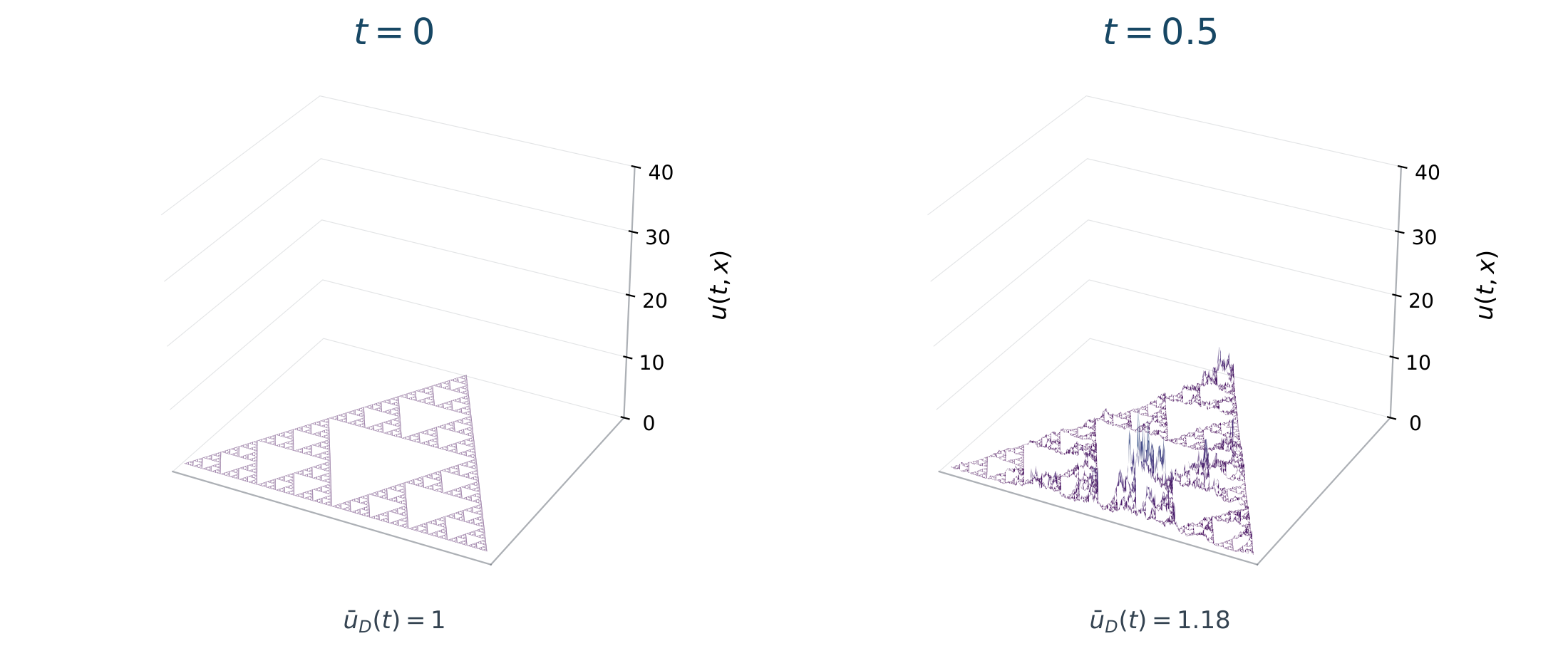
The same realization at times $t=0$ and $t=0.5$. Heights represent the unnormalized solution, with a common scale for all four panels.

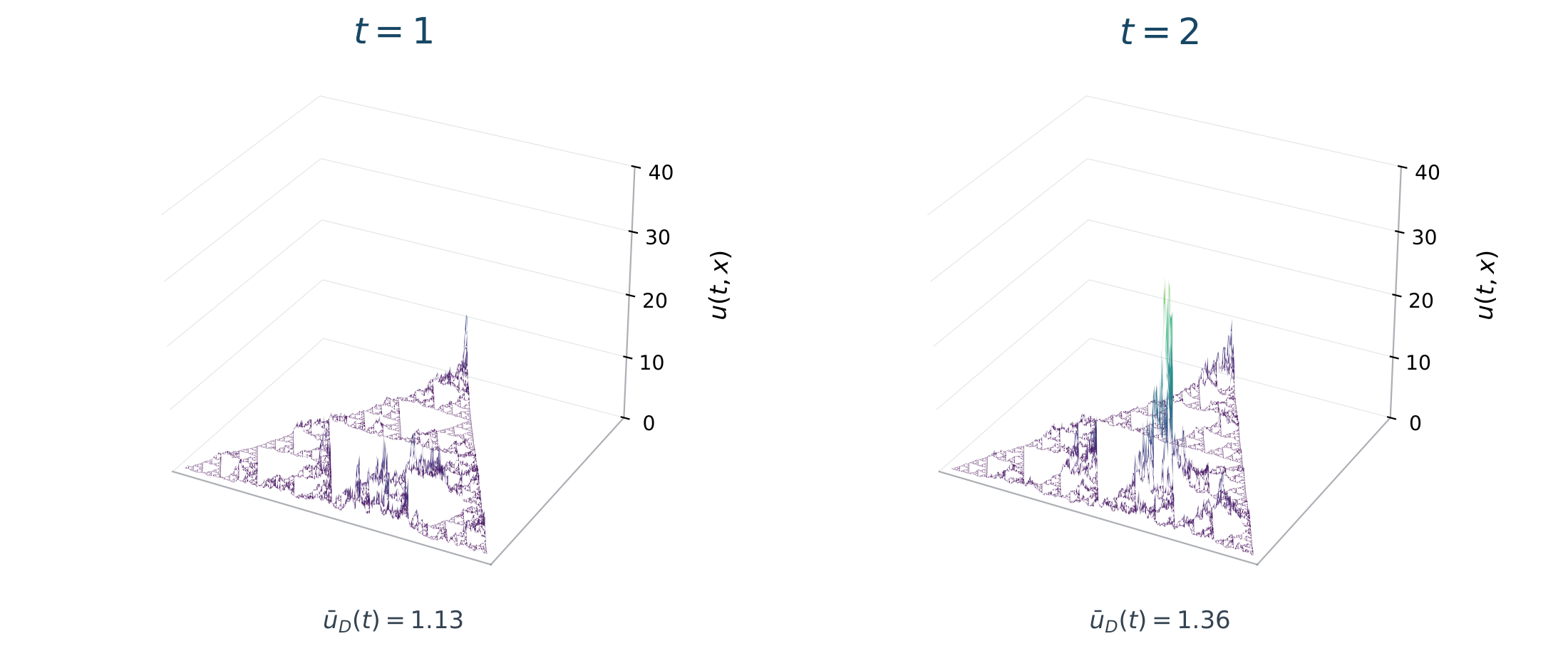
The realization at times $t=1$ and $t=2$. The numbers below the panels are spatial averages over the observation cell.

These averages approximate

At $t=2$, the largest displayed value is about $34.2$, while the spatial average is about $1.36$. The pictures illustrate spatial concentration in a finite graph approximation. The intermittency theorem concerns the asymptotic growth of ensemble moments.

The new paper contains the full statements and proofs, the scaling argument, and the details of the numerical approximation.

AI tools were only used at the end of the project when we already had a substantial manuscript in our hands. They were mostly used for polishing, proofreading, proof presentations and numerical simulations. However, ChatGPT Astra 6 discovered the approach for the existence of moments of real orders, that we then simplified later; we had a proof based on Feynman-Kac formulas that only worked for moments of integer order. ChatGPT Sol 6.1 was used in assisting the writing of this post.